Tutorial 01 — A dielectric sphere at X-band, checked against Mie

A T-matrix solver for nonspherical particles must reduce to classical Mie theory in the axis_ratio = 1 limit. That reduction is the simplest end-to-end check we can do. This tutorial builds a 1 mm water sphere at X-band, computes its scattering and extinction cross-sections via the T-matrix path, and compares against the closed-form Mie expressions shipped with rustmatrix.

import numpy as np
import matplotlib.pyplot as plt

from rustmatrix import Scatterer, mie_qsca, mie_qext, scatter
from rustmatrix.tmatrix_aux import geom_horiz_back, wl_X
from rustmatrix.refractive import m_w_10C

Build a sphere scatterer at X-band

radius_mm = 1.0
wavelength_mm = wl_X
m = m_w_10C[wl_X]

s = Scatterer(radius=radius_mm, wavelength=wavelength_mm, m=m,
              axis_ratio=1.0, ddelt=1e-4, ndgs=2)
s.set_geometry(geom_horiz_back)
S, Z = s.get_SZ()
S

array([[ 3.23494664e-02-1.33581053e-03j,  2.28305035e-25+2.05110303e-26j],
       [-2.28305035e-25-2.05110303e-26j, -3.23494664e-02+1.33581053e-03j]])

Cross-sections — T-matrix vs Mie

size_param = 2.0 * np.pi * radius_mm / wavelength_mm
sigma_sca_tm = scatter.sca_xsect(s, h_pol=True)
sigma_ext_tm = scatter.ext_xsect(s, h_pol=True)

geom = np.pi * radius_mm ** 2
sigma_sca_mie = mie_qsca(size_param, m.real, m.imag) * geom
sigma_ext_mie = mie_qext(size_param, m.real, m.imag) * geom

print(f'rel err σ_sca = {abs(sigma_sca_tm-sigma_sca_mie)/sigma_sca_mie:.2e}')
print(f'rel err σ_ext = {abs(sigma_ext_tm-sigma_ext_mie)/sigma_ext_mie:.2e}')

rel err σ_sca = 6.05e-08
rel err σ_ext = 2.86e-13

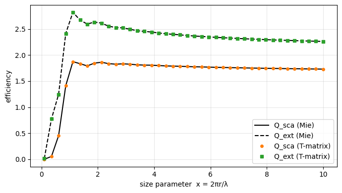
Q_sca and Q_ext across a size-parameter sweep

Plotting both curves side by side makes the Mie ripple pattern visible and confirms that the T-matrix follows it point-for-point.

xs = np.linspace(0.1, 10.0, 40)
q_sca_mie = np.array([mie_qsca(x, m.real, m.imag) for x in xs])
q_ext_mie = np.array([mie_qext(x, m.real, m.imag) for x in xs])
q_sca_tm = np.empty_like(xs)
q_ext_tm = np.empty_like(xs)
for i, x in enumerate(xs):
    r = x * wavelength_mm / (2.0 * np.pi)
    si = Scatterer(radius=r, wavelength=wavelength_mm, m=m,
                   axis_ratio=1.0, ddelt=1e-4, ndgs=2)
    si.set_geometry(geom_horiz_back)
    g = np.pi * r ** 2
    q_sca_tm[i] = scatter.sca_xsect(si) / g
    q_ext_tm[i] = scatter.ext_xsect(si) / g

fig, ax = plt.subplots(figsize=(7, 4))
ax.plot(xs, q_sca_mie, 'k-', label='Q_sca (Mie)')
ax.plot(xs, q_ext_mie, 'k--', label='Q_ext (Mie)')
ax.plot(xs, q_sca_tm, 'C1o', markersize=4, label='Q_sca (T-matrix)')
ax.plot(xs, q_ext_tm, 'C2s', markersize=4, label='Q_ext (T-matrix)')
ax.set_xlabel('size parameter  x = 2πr/λ')
ax.set_ylabel('efficiency')
ax.legend()
ax.grid(True, alpha=0.3)
fig.tight_layout();