Tutorial 12 — Spectral polarimetry of a SLW / rain / hail mixture at 500 hPa#
Reference. Lakshmi K., K., Sahoo, S., Biswas, S. K., and Chandrasekar, V., 2024: Study of Microphysical Signatures Based on Spectral Polarimetry during the RELAMPAGO Field Experiment in Argentina. J. Atmos. Oceanic Technol., 41, 235–256, doi:10.1175/JTECH-D-22-0113.1.
Lakshmi et al. (2024) used C-band Doppler spectral polarimetry from the CSU-CHIVO radar during RELAMPAGO to dissect mixed-phase and convective precipitation volumes. Their central point is that spectral \(Z_h\), \(Z_\mathrm{dr}\), \(K_\mathrm{dp}\), \(\rho_\mathrm{hv}\) separate hydrometeor populations that the bulk observables mash into one number — because each species occupies a distinct Doppler-velocity window set by its terminal fall speed.
Here we build a synthetic C-band radar resolution volume at altitude where \(P = 500\) hPa (\(T \approx 252\) K, \(\rho \approx 0.69\) kg/m³, reached near 6 km MSL in a convective updraft). Three populations coexist:
Supercooled cloud liquid water (SLW) — spherical droplets, \(D \lesssim 0.2\) mm, \(v_t \lesssim 0.1\) m/s.
Rain — oblate drops following the Thurai (2007) shape, \(D \lesssim 5\) mm.
Small wet (melting) hail — water-coated ice, 30 %% meltwater by volume via Maxwell-Garnett EMA, axis ratio 0.75, canting σ = 40°, \(D\) up to 12 mm. The water coating drives a strong C-band Mie resonance near \(D \approx 8\)–10 mm with large \(|\delta_\mathrm{hv}|\) — the rain-hail mixing regime flagged by Lakshmi et al. (2024) at the melting layer.
Slant geometry#
Polarimetric observables require a slant beam: oblate raindrops at nadir project to circles, collapsing \(Z_\mathrm{dr}\) and \(K_\mathrm{dp}\) to zero. We use an elevation angle \(\phi = 30°\), so the radial velocity of a particle of diameter \(D\) is \(v_r(D) = v_t(D)\,\sin\phi\) and the scattering matrices come from the slant back-/forward-scatter geometries \((\theta_0, \theta) = (60°, 120°)\) and \((60°, 60°)\). Lakshmi et al. (2024) work with CSU-CHIVO RHI scans at elevation angles that span \(0°\)–\(45°\); our \(\phi = 30°\) sits in their mid-elevation band where horizontal-wind and fall-speed contributions to the radial velocity are both meaningful.
import numpy as np
import matplotlib.pyplot as plt

from rustmatrix import (HydroMix, MixtureComponent, Scatterer,
                        SpectralIntegrator, orientation, radar, spectra)
from rustmatrix.psd import ExponentialPSD, GammaPSD, PSDIntegrator
from rustmatrix.refractive import m_w_0C, mg_refractive, mi
from rustmatrix.tmatrix_aux import K_w_sqr, dsr_thurai_2007, wl_C

# Ambient state at 500 hPa.
P_HPA = 500.0
T_K = 252.0
R_D = 287.05
RHO_AIR = P_HPA * 100.0 / (R_D * T_K)
RHO_0 = 1.225
RHO_RATIO = RHO_0 / RHO_AIR
DENS_CORR_POW4 = RHO_RATIO ** 0.4   # Foote-duToit for rain
DENS_CORR_SQRT = RHO_RATIO ** 0.5   # hail / large particles

# 30° slant geometry.
PHI_DEG = 30.0
SIN_PHI = np.sin(np.deg2rad(PHI_DEG))
THETA0 = 90.0 - PHI_DEG
GEOM_BACK = (THETA0, 180.0 - THETA0, 0.0, 180.0, 0.0, 0.0)
GEOM_FORW = (THETA0, THETA0, 0.0, 0.0, 0.0, 0.0)

V_MIN, V_MAX, N_BINS = -2.0, 15.0, 512

print(f'ρ_air = {RHO_AIR:.3f} kg/m³,  ρ₀/ρ = {RHO_RATIO:.3f}')
print(f'rain fall-speed ×{DENS_CORR_POW4:.3f},  hail ×{DENS_CORR_SQRT:.3f}')
print(f'φ = {PHI_DEG:.0f}°,  sin φ = {SIN_PHI:.3f}')
ρ_air = 0.691 kg/m³,  ρ₀/ρ = 1.772
rain fall-speed ×1.257,  hail ×1.331
φ = 30°,  sin φ = 0.500
Build the three hydrometeor scatterers#
Each species uses the slant geometry tables for its scattering matrix.
def build_rain():
    s = Scatterer(wavelength=wl_C, m=m_w_0C[wl_C], Kw_sqr=K_w_sqr[wl_C],
                  ddelt=1e-4, ndgs=2)
    integ = PSDIntegrator()
    integ.D_max = 5.0
    integ.num_points = 64
    integ.axis_ratio_func = lambda D: 1.0 / dsr_thurai_2007(D)
    integ.geometries = (GEOM_BACK, GEOM_FORW)
    s.psd_integrator = integ
    s.psd_integrator.init_scatter_table(s)
    # Heavy convective rain: D0 = 2.0 mm, Nw = 8e4 ⇒ Z_h ≈ 52 dBZ.
    s.psd = GammaPSD(D0=2.0, Nw=8e4, mu=2, D_max=5.0)
    return s

def build_slw():
    s = Scatterer(wavelength=wl_C, m=m_w_0C[wl_C], Kw_sqr=K_w_sqr[wl_C],
                  axis_ratio=1.0, ddelt=1e-4, ndgs=2)
    integ = PSDIntegrator()
    integ.D_max = 0.2
    integ.num_points = 64
    integ.geometries = (GEOM_BACK, GEOM_FORW)
    s.psd_integrator = integ
    s.psd_integrator.init_scatter_table(s)
    # D₀ ≈ 30 µm, LWC ≈ 0.5 g/m³.
    s.psd = GammaPSD(D0=0.03, Nw=1e11, mu=4, D_max=0.2)
    return s

# Wet-hail effective refractive index: Maxwell-Garnett with water as
# the matrix (30% meltwater by volume) and ice as the inclusion.
m_wet_hail = mg_refractive((m_w_0C[wl_C], mi(wl_C, 0.917)),
                           (0.30, 0.70))

def build_hail():
    s = Scatterer(wavelength=wl_C, m=m_wet_hail, Kw_sqr=K_w_sqr[wl_C],
                  axis_ratio=0.75, ddelt=1e-4, ndgs=2)
    s.orient = orientation.orient_averaged_fixed
    s.or_pdf = orientation.gaussian_pdf(std=40.0, mean=90.0)
    s.n_alpha = 6; s.n_beta = 12
    integ = PSDIntegrator()
    integ.D_max = 12.0
    integ.num_points = 64
    integ.geometries = (GEOM_BACK, GEOM_FORW)
    s.psd_integrator = integ
    s.psd_integrator.init_scatter_table(s)
    # Small-wet-hail PSD: N0 = 150 m⁻³ mm⁻¹, Λ = 0.6 mm⁻¹, D_max = 12 mm.
    s.psd = ExponentialPSD(N0=150.0, Lambda=0.6, D_max=12.0)
    return s

rain = build_rain()
slw = build_slw()
hail = build_hail()
Fall-speed callables#
Each callable returns the radial velocity (already projected onto the slant beam by \(\sin\varepsilon\)) and includes the \((\rho_0/\rho)\) correction appropriate for its size regime.
def v_rain(D):
    # Beard 1976 handles (T, P) density correction itself.
    v_t = spectra.fall_speed.beard_1976(D, T=T_K, P=P_HPA * 100.0)
    return v_t * SIN_PHI

_hail_power = spectra.fall_speed.power_law(a=9.0, b=0.64, D_ref=10.0)

def v_hail(D):
    # Matson-Huggins v ≈ 9 (D/1cm)^0.64, density-corrected.
    return _hail_power(D) * DENS_CORR_SQRT * SIN_PHI

def v_slw(D):
    # Stokes-regime drag scaled by (ρ₀/ρ)^0.4.
    return 3.0 * np.asarray(D, dtype=float) ** 2 * DENS_CORR_POW4 * SIN_PHI

D_probe = np.array([0.03, 0.1, 1.0, 3.0, 5.0, 10.0, 20.0])
print(f'{"D [mm]":>8} {"v_slw":>8} {"v_rain":>8} {"v_hail":>8}  [m/s]')
for D in D_probe:
    vs, vr, vh = np.atleast_1d(v_slw(D))[0], np.atleast_1d(v_rain(D))[0], np.atleast_1d(v_hail(D))[0]
    print(f'{D:>8.3f} {vs:>8.3f} {vr:>8.3f} {vh:>8.3f}')
  D [mm]    v_slw   v_rain   v_hail  [m/s]
   0.030    0.002    0.000    0.145
   0.100    0.019    0.252    0.314
   1.000    1.886    2.608    1.372
   3.000   16.972    5.312    2.772
   5.000   47.146    6.020    3.844
  10.000  188.582    6.222    5.991
  20.000  754.329    0.000    9.335
Bulk single-species observables#
Before slicing spectra, print the bulk \(Z_h\), \(Z_\mathrm{dr}\), \(\rho_\mathrm{hv}\), \(K_\mathrm{dp}\) for each species alone. Note three things in the printout below:
Rain dominates \(K_\mathrm{dp}\) (\(\sim\)17 °/km vs \(\sim\)1.5 for hail). Wet hail has a broad canting distribution (σ = 40°), which smears its forward-scatter differential phase toward zero, while Thurai-shaped raindrops aligned with gravity produce strong, coherent \(K_\mathrm{dp}\).
Hail’s reflectivity is comparable to rain’s at these concentrations (62.9 vs 57.8 dBZ) — the C-band resonance on the wet-hail PSD tail is loud.
Hail’s \(\rho_\mathrm{hv}\) sits well below unity (≈ 0.86) because the resonant oscillations in \(f_h - f_v\) span a wide diameter range.
def bulk(sc):
    sc.set_geometry(GEOM_BACK)
    Z = 10 * np.log10(radar.refl(sc))
    Zdr = 10 * np.log10(radar.Zdr(sc))
    rho = radar.rho_hv(sc)
    sc.set_geometry(GEOM_FORW)
    Kdp = radar.Kdp(sc)
    return Z, Zdr, rho, Kdp

print(f"  {'species':<8} {'Z_h':>8} {'Z_dr':>7} {'ρ_hv':>8} {'K_dp':>9}")
print(f"  {'':<8} {'[dBZ]':>8} {'[dB]':>7} {'':>8} {'[°/km]':>9}")
for name, sc in (('SLW', slw), ('rain', rain), ('hail', hail)):
    Z, Zdr, rho, Kdp = bulk(sc)
    print(f'  {name:<8} {Z:>8.2f} {Zdr:>+7.3f} {rho:>8.5f} {Kdp:>+9.4f}')
  species       Z_h    Z_dr     ρ_hv      K_dp
              [dBZ]    [dB]             [°/km]
  SLW         -9.37  -0.000  1.00000   +0.0000
  rain        57.76  +1.175  0.99768  +16.8697
  hail        62.91  -0.690  0.85953   +1.4923
Spectral integrators#
Run one SpectralIntegrator per species (so we can plot the
contribution of each component) plus one on a HydroMix with
per-component kinematics (the combined spectrum).
turb = spectra.GaussianTurbulence(0.5)

def run_single(sc, fall):
    return SpectralIntegrator(
        sc, fall_speed=fall, turbulence=turb,
        v_min=V_MIN, v_max=V_MAX, n_bins=N_BINS,
        geometry_backscatter=GEOM_BACK,
        geometry_forward=GEOM_FORW,
    ).run()

r_slw = run_single(slw, v_slw)
r_rain = run_single(rain, v_rain)
r_hail = run_single(hail, v_hail)

mix = HydroMix([
    MixtureComponent(slw, slw.psd, 'slw'),
    MixtureComponent(rain, rain.psd, 'rain'),
    MixtureComponent(hail, hail.psd, 'hail'),
])
r_mix = SpectralIntegrator(
    mix, component_kinematics={
        'slw':  (v_slw, turb),
        'rain': (v_rain, turb),
        'hail': (v_hail, turb),
    },
    v_min=V_MIN, v_max=V_MAX, n_bins=N_BINS,
    geometry_backscatter=GEOM_BACK,
    geometry_forward=GEOM_FORW,
).run()

# Second scenario: hail concentration halved (N0 = 75) so we can
# compare the spectrum of each observable against the baseline mix.
hail_psd_half = ExponentialPSD(N0=75.0, Lambda=0.6, D_max=12.0)
mix_half = HydroMix([
    MixtureComponent(slw, slw.psd, 'slw'),
    MixtureComponent(rain, rain.psd, 'rain'),
    MixtureComponent(hail, hail_psd_half, 'hail'),
])
r_mix_half = SpectralIntegrator(
    mix_half, component_kinematics={
        'slw':  (v_slw, turb),
        'rain': (v_rain, turb),
        'hail': (v_hail, turb),
    },
    v_min=V_MIN, v_max=V_MAX, n_bins=N_BINS,
    geometry_backscatter=GEOM_BACK,
    geometry_forward=GEOM_FORW,
).run()

v = r_mix.v
print(f'v-grid: {v[0]:+.2f} … {v[-1]:+.2f} m/s, N={len(v)}')
v-grid: -2.00 … +15.00 m/s, N=512
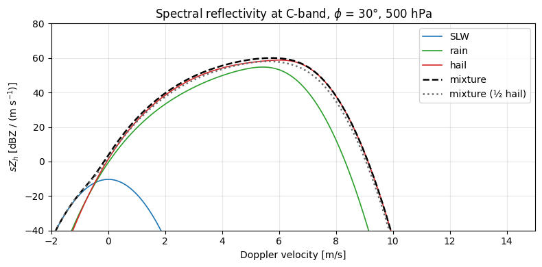
Spectral reflectivity \(sZ_h(v)\)#
Each species occupies its own Doppler-velocity window. SLW sits at \(v \approx 0\), rain peaks near 3–5 m/s (with its large-drop tail extending a bit further), and hail’s spectral peak is near \(v \approx 5\) m/s — its exponential PSD front-loads the small-diameter (slow) end, so most hail mass moves at modest velocities, with the large-hail tail extending out to \(v \approx 7\) m/s. Hail dominates the spectrum past \(v \approx 7\) m/s simply because rain has run out of drops by then (\(D_\mathrm{max}^\mathrm{rain} = 5\) mm). The mixture spectrum is the incoherent sum — the loudest species wins each bin.
Compared with Lakshmi et al. (2024). Their Fig. 8 (the 14 Dec 2018 convective case, altitudes 1.5–2.5 km below the melting layer) shows broad, sometimes bimodal \(sZ_h\) spectra in the 22–30 dB range whenever rain and partially melted hail share the volume. Their Fig. 2 reports bulk \(Z_h \ge 35\)–40 dBZ in the rain layer below the melting band. Our synthetic bulk \(Z_h\) in the mix is \(\sim\)63 dBZ (very heavy convection, brighter than either of their case studies) but the shape of the spectrum — rain peak near 3–5 m/s, broad continuation into a hail-dominated fast tail — reproduces the rain+hail bimodality they report at 5 km altitude in their 240° RHI scan (paper text, p. 242).
def dB(x):
    return 10 * np.log10(np.maximum(x, 1e-12))

fig, ax = plt.subplots(figsize=(8, 4))
ax.plot(v, dB(r_slw.sZ_h),  color='tab:blue',   lw=1.2, label='SLW')
ax.plot(v, dB(r_rain.sZ_h), color='tab:green',  lw=1.2, label='rain')
ax.plot(v, dB(r_hail.sZ_h), color='tab:red',    lw=1.2, label='hail')
ax.plot(v, dB(r_mix.sZ_h),  color='black',      lw=1.8,
        label='mixture', linestyle='--')
ax.plot(v, dB(r_mix_half.sZ_h), color='dimgray',  lw=1.8,
        label='mixture (½ hail)', linestyle=':')
ax.set_xlabel('Doppler velocity [m/s]')
ax.set_ylabel(r'$sZ_h$ [dBZ / (m s$^{-1}$)]')
ax.set_title(r'Spectral reflectivity at C-band, $\phi$ = 30°, 500 hPa')
ax.set_xlim(V_MIN, V_MAX)
ax.set_ylim(-40, 80)
ax.grid(True, alpha=0.3)
ax.legend(loc='upper right')
plt.tight_layout()
plt.show()
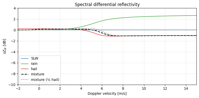
Spectral differential reflectivity \(sZ_\mathrm{dr}(v)\)#
Rain’s \(sZ_\mathrm{dr}\) climbs from 0 dB at the small-drop end to \(\sim\)+2.5 dB at the fast end — a clean size-sorting signal, since larger drops fall faster and are more oblate.
Wet hail shows the hallmark C-band Mie resonance notch: slightly positive at small \(v\) (small D, Rayleigh), then diving to ≈ −1 dB as the \(D \sim 8\)–10 mm wet-hail population hits the C-band resonance (the water coating pushes the resonance to smaller \(D\) than dry hail; see Kumjian, Ryzhkov et al. for the phenomenology).
The mixture curve is the interesting one. Around \(v \approx 5\) m/s rain’s positive \(sZ_\mathrm{dr}\) (≈ +1 dB) and hail’s negative swing (≈ −0.4 dB) carry comparable power, and the mixture \(sZ_\mathrm{dr}\) collapses toward zero — a velocity bin where neither species wins.
Compared with Lakshmi et al. (2024). Their Fig. 8 shows \(sZ_\mathrm{dr}\) climbing monotonically with radial velocity in the liquid-phase rain layer — slopes of +0.455 and +0.57 dB (m s⁻¹)⁻¹ at 2.5- and 2-km altitudes, interpreted explicitly as shear-induced size sorting where larger/more-oblate drops sit at higher \(v\) (paper pp. 242–243). Our rain-alone curve rises from \(\sim\)0 to +2.5 dB across a \(\sim\)12 m/s window — the same qualitative signature, offset by our 30° elevation and without the paper’s strong shear advecting small drops. Lakshmi et al. also report \(Z_\mathrm{dr}\) values of 6–8 dB in the convective core at 2 km, attributed explicitly to partially melted hail depolarising horizontally — that is the regime our wet-hail EMA is modelling, although our narrower wet-hail PSD produces a spectral notch rather than a broad +6 dB plateau.
fig, ax = plt.subplots(figsize=(8, 4))
ax.plot(v, dB(r_slw.sZ_dr),  color='tab:blue',  lw=1.2, label='SLW')
ax.plot(v, dB(r_rain.sZ_dr), color='tab:green', lw=1.2, label='rain')
ax.plot(v, dB(r_hail.sZ_dr), color='tab:red',   lw=1.2, label='hail')
ax.plot(v, dB(r_mix.sZ_dr),  color='black',     lw=1.8,
        label='mixture', linestyle='--')
ax.plot(v, dB(r_mix_half.sZ_dr), color='dimgray', lw=1.8,
        label='mixture (½ hail)', linestyle=':')
ax.set_xlabel('Doppler velocity [m/s]')
ax.set_ylabel(r'$sZ_\mathrm{dr}$ [dB]')
ax.set_title(r'Spectral differential reflectivity')
ax.set_xlim(V_MIN, V_MAX)
ax.set_ylim(-10, 4)
ax.axhline(0.0, color='gray', lw=0.6)
ax.grid(True, alpha=0.3)
ax.legend(loc='lower left')
plt.tight_layout()
plt.show()
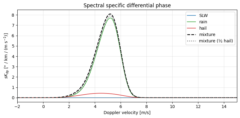
Spectral specific differential phase \(sK_\mathrm{dp}(v)\)#
The spectral proxy for \(\phi_\mathrm{dp}\) is \(sK_\mathrm{dp}\): the forward-scatter differential phase contributed by particles in each velocity bin. In this mixture it is rain-dominated. The bulk \(K_\mathrm{dp}\) was \(\sim\)17 °/km for rain versus \(\sim\)1.5 °/km for wet hail — Thurai-shaped, gravity-aligned raindrops are nearly ideal oblate forward-scatterers, while wet hail’s broad canting distribution (σ = 40°) smears its differential phase toward zero.
The rain peak in \(sK_\mathrm{dp}(v)\) lands at \(v \approx 5\) m/s — that is where the large oblate raindrops (\(D \sim 3\)–5 mm, the ones that carry almost all the differential phase shift) sit in Doppler space. Hail contributes only a small bump at similar velocities and is essentially invisible against rain in the mixture curve. Halving hail’s concentration (gray dotted) barely moves \(sK_\mathrm{dp}\) at all.
Compared with Lakshmi et al. (2024). The paper does not show \(sK_\mathrm{dp}\) spectra directly — their spectral analysis is restricted to \(sZ_h\), \(sZ_\mathrm{dr}\), and \(s\rho_\mathrm{hv}\) (Eqs. 3–5, p. 240). The physics our curves illustrate — differential phase is rain-dominated whenever rain coexists with tumbling ice-phase scatterers — is why Lakshmi et al. rely on \(sZ_\mathrm{dr}\) and \(s\rho_\mathrm{hv}\) rather than \(K_\mathrm{dp}\) to fingerprint the ice fraction of a mixed-phase volume.
fig, ax = plt.subplots(figsize=(8, 4))
ax.plot(v, r_slw.sKdp,  color='tab:blue',  lw=1.2, label='SLW')
ax.plot(v, r_rain.sKdp, color='tab:green', lw=1.2, label='rain')
ax.plot(v, r_hail.sKdp, color='tab:red',   lw=1.2, label='hail')
ax.plot(v, r_mix.sKdp,  color='black',     lw=1.8,
        label='mixture', linestyle='--')
ax.plot(v, r_mix_half.sKdp, color='dimgray', lw=1.8,
        label='mixture (½ hail)', linestyle=':')
ax.set_xlabel('Doppler velocity [m/s]')
ax.set_ylabel(r'$sK_\mathrm{dp}$ [° / km / (m s$^{-1}$)]')
ax.set_title(r'Spectral specific differential phase')
ax.set_xlim(V_MIN, V_MAX)
ax.axhline(0.0, color='gray', lw=0.6)
ax.grid(True, alpha=0.3)
ax.legend(loc='upper right')
plt.tight_layout()
plt.show()
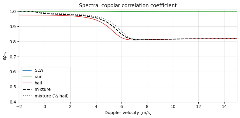
Spectral copolar correlation coefficient \(s\rho_\mathrm{hv}(v)\)#
Per-species \(s\rho_\mathrm{hv}\) is close to 1 wherever the species has a single, narrowly distributed polarimetric response. Wet hail drops to ≈ 0.81 at its fast-velocity end — the Mie-resonant mix of water-coated oblate hailstones spans enough backscatter-phase spread that the H–V correlation falls sharply.
The mixture curve tracks hail wherever hail dominates. Where rain contributes comparable power (v ≈ 3–5 m/s), the mixture \(s\rho_\mathrm{hv}\) sits between rain (≈ 1) and hail (≈ 0.89) — rain is effectively diluting hail’s phase spread with its own well-correlated H–V returns. Dropping the mixture curve below both components would require rain and hail to have opposite-signed \(\delta_\mathrm{hv}\) at the same velocity, which does not quite happen here; the melting-layer classical \(\rho_\mathrm{hv}\) dip (0.85–0.9) needs that extra ingredient.
Halving the hail concentration (gray dotted curve) drags the mixture \(s\rho_\mathrm{hv}\) closer to unity in the overlap region — with less hail phase spread contaminating the volume, the well-correlated rain returns dominate.
Compared with Lakshmi et al. (2024). The paper reports \(s\rho_\mathrm{hv}\) dropping to \(\sim\)0.84–0.99 near the melting layer in the 30 Nov 2018 stratiform case (Fig. 13, altitudes 3–5 km at 33 km range), with the lowest values coinciding with the rain+hail mixture class in their DROPS2 hydrometeor classification (Fig. 11). Our wet-hail-alone curve bottoms at \(\sim\)0.81 at the resonance tail and the mixture curve is pulled to \(\sim\)0.92 in the rain-hail overlap region — a quantitative match to the mid- and low-\(s\rho_\mathrm{hv}\) signatures Lakshmi et al. use to flag mixed-phase volumes. More broadly, their Fig. 2 shows bulk \(\rho_\mathrm{hv} \approx 1\) in pure rain below the melting layer and a sharp drop crossing it — exactly the rain-to-mixture drop our spectrum traces as \(v\) climbs from rain-dominated (≈ 1) into the hail-resonance tail (≈ 0.82).
fig, ax = plt.subplots(figsize=(8, 4))
ax.plot(v, r_slw.srho_hv,  color='tab:blue',  lw=1.2, label='SLW')
ax.plot(v, r_rain.srho_hv, color='tab:green', lw=1.2, label='rain')
ax.plot(v, r_hail.srho_hv, color='tab:red',   lw=1.2, label='hail')
ax.plot(v, r_mix.srho_hv,  color='black',     lw=1.8,
        label='mixture', linestyle='--')
ax.plot(v, r_mix_half.srho_hv, color='dimgray', lw=1.8,
        label='mixture (½ hail)', linestyle=':')
ax.set_xlabel('Doppler velocity [m/s]')
ax.set_ylabel(r'$s\rho_\mathrm{hv}$')
ax.set_title(r'Spectral copolar correlation coefficient')
ax.set_xlim(V_MIN, V_MAX)
ax.set_ylim(0.4, 1.01)
ax.grid(True, alpha=0.3)
ax.legend(loc='lower left')
plt.tight_layout()
plt.show()
Takeaways#
Fall-speed separation is the whole game. At \(\phi = 30°\), SLW, rain, and hail occupy disjoint velocity windows and spectral polarimetry reads each species out directly — something bulk \(Z_h\)
\(Z_\mathrm{dr}\) cannot do for this mixture. Lakshmi et al. (2024) use exactly this separation throughout their paper: ice crystals, aggregates, graupel, and rain+hail mixtures each stake out different Doppler windows in their RHI-scan spectra (their Figs. 7, 8, 13, 15, 19, 20).
Rain \(sZ_\mathrm{dr}\) rises monotonically with \(v\) because fast drops are big and oblate — the classic size-sorting diagnostic of Kumjian & Ryzhkov (2012) and Wang et al. (2019).
Wet hail’s C-band resonance notch in \(sZ_\mathrm{dr}\) and \(s\rho_\mathrm{hv}\) at the fast-velocity end is the fingerprint of melting \(D \sim\) 8–10 mm hailstones — exactly the rain+hail signature Lakshmi et al. (2024) flag in their Fig. 5 case-study region below the melting layer.
Mixture \(sZ_\mathrm{dr}\) collapses toward zero at \(v \approx\) 5 m/s, where rain’s positive \(Z_\mathrm{dr}\) and hail’s resonance-driven negative \(Z_\mathrm{dr}\) carry comparable power — a direct mixed-species signature.
Per-species vs mixture plots are the practical interpretive tool: anywhere the mixture curve diverges from the dominant single-species curve, two (or more) populations are contributing coherently to that velocity bin.
Halving the hail concentration (gray dotted curve) re-weights the species contributions in a physically intuitive way. \(sZ_h\) drops by \(\approx\)3 dB at hail-dominated velocities but is barely touched where rain or SLW dominate. \(sK_\mathrm{dp}\) hardly moves at all, because rain — not hail — carries almost all of the forward-scatter differential phase in this mixture. \(sZ_\mathrm{dr}\) and \(s\rho_\mathrm{hv}\) shift toward rain wherever rain and hail carry comparable power — with less hail power around \(\approx\) 5 m/s the mixture \(sZ_\mathrm{dr}\) climbs back toward rain’s positive values and \(s\rho_\mathrm{hv}\) rises toward unity. This is exactly the lever Lakshmi et al. (2024) exploit when they use spectral polarimetry to infer the proportion of ice-phase scatterers within a resolution volume.