Tutorial 02 — Single-drop polarimetric response at S/C/X bands#
Falling raindrops are flattened by drag; larger drops are more oblate (Thurai et al. 2007). That shape anisotropy imprints four distinct signatures on dual-polarisation radar data:
Z_h grows as D⁶ in the Rayleigh regime and then walks out of it — earliest at X-band, latest at S-band.
Z_dr rises with D because oblateness grows with D; the wavelength dependence exposes C-band’s resonance bump near D ≈ 5 mm.
K_dp scales with Re(f_h(0) − f_v(0)) — strictly stronger at shorter wavelengths; X-band K_dp per drop is ≈ 2× C-band and ≈ 4× S-band.
LDR — linear depolarisation ratio — is set by the canting distribution. Here we model a σ = 5° Gaussian wobble around the flat-lying orientation to produce realistic rain LDR in the −30 to −25 dB range for 5+ mm drops.
This notebook sweeps drop equivalent diameter D = 0.1–8 mm at S, C, and X bands and plots all four observables. We report Z_h and K_dp per drop/m³ so multiplying by the drop concentration N [m⁻³] gives the usual bulk observables.
import numpy as np
import matplotlib.pyplot as plt

from rustmatrix import Scatterer, orientation, radar, scatter
from rustmatrix.tmatrix_aux import (K_w_sqr, dsr_thurai_2007,
                                      geom_horiz_back, geom_horiz_forw,
                                      wl_C, wl_S, wl_X)
from rustmatrix.refractive import m_w_10C

BANDS = [('S', wl_S, 'C0'), ('C', wl_C, 'C1'), ('X', wl_X, 'C2')]
D_GRID = np.linspace(0.1, 8.0, 40)
CANTING_STD_DEG = 5.0
Build the drop and run the sweep#
One Scatterer per (D, λ) point, with a σ = 5° Gaussian canting
PDF around β = 0° (flat-lying oblate drop with modest turbulent
wobble). Backscatter geometry gives Z_h, Z_dr, and LDR; forward
geometry gives K_dp.
def build_drop(D_mm, wl):
    s = Scatterer(radius=D_mm/2, wavelength=wl, m=m_w_10C[wl],
                  axis_ratio=1.0/dsr_thurai_2007(D_mm),
                  Kw_sqr=K_w_sqr[wl], ddelt=1e-4, ndgs=2)
    s.orient = orientation.orient_averaged_fixed
    s.or_pdf = orientation.gaussian_pdf(std=CANTING_STD_DEG, mean=0.0)
    s.n_alpha = 6; s.n_beta = 12
    return s

def sweep(wl):
    Zh = np.empty_like(D_GRID); Zdr = np.empty_like(D_GRID)
    Kdp = np.empty_like(D_GRID); LDR = np.empty_like(D_GRID)
    for i, D in enumerate(D_GRID):
        s = build_drop(D, wl)
        s.set_geometry(geom_horiz_back)
        Zh[i]  = 10*np.log10(max(radar.refl(s, h_pol=True), 1e-30))
        Zdr[i] = 10*np.log10(max(radar.Zdr(s), 1e-30))
        LDR[i] = 10*np.log10(max(scatter.ldr(s, h_pol=True), 1e-30))
        s.set_geometry(geom_horiz_forw)
        Kdp[i] = radar.Kdp(s)
    return dict(Zh=Zh, Zdr=Zdr, Kdp=Kdp, LDR=LDR)

data = {name: sweep(wl) for name, wl, _ in BANDS}
Plot all four observables vs. D#
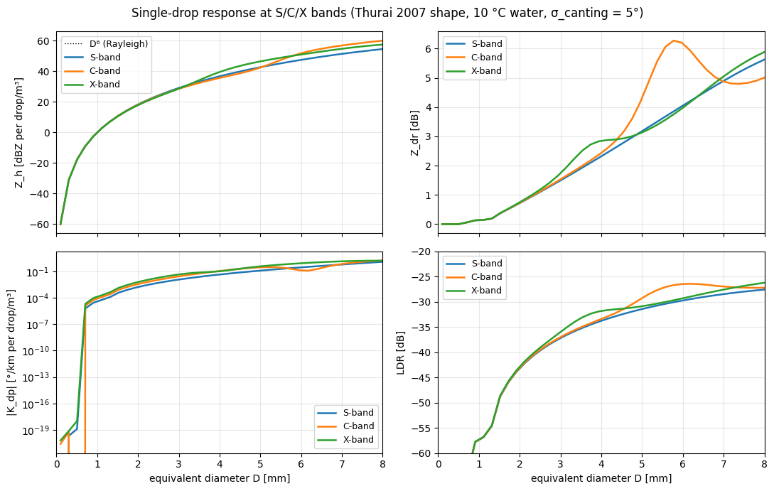
Top-left Z_h tracks the D⁶ line until it bends: X-band breaks earliest (shortest λ, smallest χ = πD/λ needed), S-band last. Top-right Z_dr rises monotonically; the C-band curve bumps above X and S around D ≈ 5 mm — the well-known C-band raindrop resonance. Bottom-left K_dp ordering is X > C > S at every D. Bottom-right LDR is a clean fingerprint of the canting distribution and rises smoothly with D once the drop is oblate enough to leak cross-pol power.
fig, axes = plt.subplots(2, 2, figsize=(11, 7), sharex=True)

ref_D = D_GRID[(D_GRID > 0.5) & (D_GRID < 2.5)]
rayleigh = 10*np.log10(ref_D**6) + (data['S']['Zh'][10] - 10*np.log10(D_GRID[10]**6))
axes[0, 0].plot(ref_D, rayleigh, 'k:', lw=1, label='D⁶ (Rayleigh)')
for name, _, c in BANDS:
    axes[0, 0].plot(D_GRID, data[name]['Zh'], color=c, lw=1.8, label=f'{name}-band')
axes[0, 0].set_ylabel('Z_h [dBZ per drop/m³]')
axes[0, 0].legend(fontsize=9)

for name, _, c in BANDS:
    axes[0, 1].plot(D_GRID, data[name]['Zdr'], color=c, lw=1.8, label=f'{name}-band')
axes[0, 1].set_ylabel('Z_dr [dB]')
axes[0, 1].legend(fontsize=9)

for name, _, c in BANDS:
    axes[1, 0].semilogy(D_GRID, np.abs(data[name]['Kdp']),
                         color=c, lw=1.8, label=f'{name}-band')
axes[1, 0].set_ylabel('|K_dp| [°/km per drop/m³]')
axes[1, 0].legend(fontsize=9)

for name, _, c in BANDS:
    axes[1, 1].plot(D_GRID, data[name]['LDR'], color=c, lw=1.8, label=f'{name}-band')
axes[1, 1].set_ylim(-60, -20)
axes[1, 1].set_ylabel('LDR [dB]')
axes[1, 1].legend(fontsize=9)

for ax in axes.flat:
    ax.set_xlim(0, 8)
    ax.grid(True, alpha=0.3)
axes[1, 0].set_xlabel('equivalent diameter D [mm]')
axes[1, 1].set_xlabel('equivalent diameter D [mm]')
fig.suptitle(f'Single-drop response at S/C/X bands '
             f'(Thurai 2007 shape, 10 °C water, σ_canting = {CANTING_STD_DEG:.0f}°)')
fig.tight_layout();
Spot values at canonical diameters#
Six diameters span the regime map: 0.5 mm (nearly spherical, pure Rayleigh), 1–3 mm (moderate oblateness, still Rayleigh at S/C), 5 mm (C-band resonance territory), and 7 mm (well into non-Rayleigh at all three bands).
rows = (0.5, 1.0, 2.0, 3.0, 5.0, 7.0)
idx = [int(np.argmin(np.abs(D_GRID - D))) for D in rows]
for obs, fmt in (('Zh', '{:+7.2f}'), ('Zdr', '{:+7.3f}'),
                 ('Kdp', '{:+7.2e}'), ('LDR', '{:+7.2f}')):
    label = {'Zh': 'Z_h [dBZ]', 'Zdr': 'Z_dr [dB]',
             'Kdp': 'K_dp [°/km]', 'LDR': 'LDR [dB]'}[obs]
    header = '  '.join(f'D={D:>3.1f}' for D in rows)
    print(f'{label:<14}  {header}')
    for name, _, _ in BANDS:
        row = data[name][obs][idx]
        cells = '  '.join(fmt.format(v) for v in row)
        print(f'  {name}-band        {cells}')
    print()
Z_h [dBZ]       D=0.5  D=1.0  D=2.0  D=3.0  D=5.0  D=7.0
  S-band         -17.79    -2.41   +17.21   +28.43   +42.40   +51.28
  C-band         -17.81    -2.45   +17.03   +27.92   +42.01   +56.74
  X-band         -17.83    -2.51   +16.79   +27.93   +46.21   +54.61

Z_dr [dB]       D=0.5  D=1.0  D=2.0  D=3.0  D=5.0  D=7.0
  S-band         -0.000   +0.129   +0.661   +1.443   +3.146   +4.889
  C-band         -0.000   +0.129   +0.669   +1.479   +4.190   +4.880
  X-band         -0.000   +0.130   +0.686   +1.656   +3.111   +5.039

K_dp [°/km]     D=0.5  D=1.0  D=2.0  D=3.0  D=5.0  D=7.0
  S-band        +1.29e-19  +2.75e-05  +1.33e-03  +1.03e-02  +1.13e-01  +5.76e-01
  C-band        +0.00e+00  +5.75e-05  +2.85e-03  +2.35e-02  +2.73e-01  +6.55e-01
  X-band        +1.03e-18  +9.35e-05  +4.84e-03  +3.97e-02  +3.45e-01  +1.33e+00

LDR [dB]        D=0.5  D=1.0  D=2.0  D=3.0  D=5.0  D=7.0
  S-band        -300.00   -57.79   -43.87   -37.47   -31.52   -28.49
  C-band        -300.00   -57.77   -43.77   -37.28   -29.46   -26.97
  X-band        -300.00   -57.72   -43.56   -36.38   -30.93   -27.61