Tutorial 07 — W-band Mie Doppler spectrum in convective rain (Kollias 2002)

Reference: Kollias, P., Albrecht, B. A., and Marks Jr., F. D., 2002. Cloud radar observations of vertical drafts and microphysics in convective rain, J. Geophys. Res., 107 (doi:10.1029/2001JD002033).

At 94 GHz the raindrop backscattering cross-section σ_b(D) is no longer Rayleigh — it rings through a sequence of Mie maxima and minima. Because each drop falls at a deterministic terminal velocity v_t(D), these Mie features map directly onto the observed Doppler spectrum: the first Mie minimum appears at v ≈ 5.9 m/s in still air, and any displacement of that feature from its theoretical location is a direct measurement of the mean vertical air motion — independent of the drop-size distribution. This notebook reproduces the paper’s Figures 1–3 and demonstrates the air-motion retrieval.

import numpy as np
import matplotlib.pyplot as plt

from rustmatrix import Scatterer, SpectralIntegrator, radar, spectra
from rustmatrix.psd import ExponentialPSD, PSDIntegrator
from rustmatrix.refractive import m_w_20C
from rustmatrix.tmatrix_aux import (K_w_sqr, dsr_thurai_2007,
                                      geom_vert_back, wl_W)

Figure 1 — single-drop σ_b(D) at 94 GHz

Each drop’s backscatter cross-section at vertical incidence, as a function of its equivalent diameter D. The Rayleigh D⁶ regime holds only below about 0.7 mm; beyond that the curve oscillates through distinct Mie resonances.

def build_drop(D_mm, oblate=True):
    axis_ratio = 1.0 / dsr_thurai_2007(D_mm) if oblate else 1.0
    s = Scatterer(radius=D_mm/2, wavelength=wl_W, m=m_w_20C[wl_W],
                  Kw_sqr=K_w_sqr[wl_W], axis_ratio=axis_ratio,
                  ddelt=1e-4, ndgs=2)
    s.set_geometry(geom_vert_back)
    return s

D_grid = np.linspace(0.05, 5.0, 400)    # mm
sigma_b_obl = np.array([radar.radar_xsect(build_drop(D, True))
                        for D in D_grid])
sigma_b_sph = np.array([radar.radar_xsect(build_drop(D, False))
                        for D in D_grid])

fig, ax = plt.subplots(figsize=(7, 4))
ax.semilogy(D_grid, sigma_b_obl, 'C0-', label='oblate (Thurai 2007)')
ax.semilogy(D_grid, sigma_b_sph, 'k--', label='sphere')
ax.set_xlabel('diameter D [mm]')
ax.set_ylabel(r'$\sigma_b$ [mm²]')
ax.set_title('Figure 1 — single-drop backscatter at 94 GHz, vertical incidence')
ax.legend(); ax.grid(True, which='both', alpha=0.3)
fig.tight_layout();

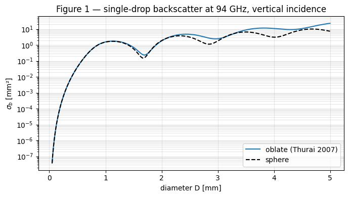
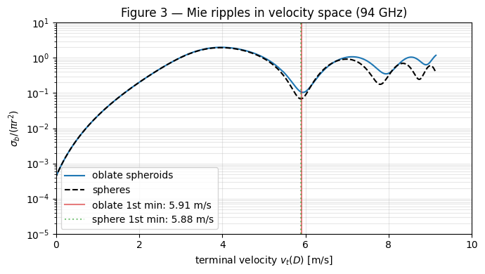
Figure 3 — Mie oscillations mapped to terminal velocity

Plotting σ_b / (π r²) versus the drop’s terminal fall speed collapses the Mie ripple structure into the velocity coordinate the radar actually measures. Oblate drops fall slightly faster than the spheres of the same equivalent diameter, so their first Mie minimum lands at v ≈ 5.95 m/s instead of 5.88 m/s — a 7 cm/s shift that matters when you’re using it as a zero-air-motion fiducial.

fall = spectra.fall_speed.atlas_srivastava_sekhon_1973
v_t = fall(D_grid)
r_mm = D_grid / 2.0
norm = np.pi * r_mm ** 2

def first_min(D, sigma_b):
    mask = (D > 1.3) & (D < 2.2)
    i = np.argmin(sigma_b[mask])
    return D[mask][i], v_t[mask][i]

D_min_obl, v_min_obl = first_min(D_grid, sigma_b_obl)
D_min_sph, v_min_sph = first_min(D_grid, sigma_b_sph)
print(f'First Mie minimum, oblate: D = {D_min_obl:.3f} mm, '
      f'v = {v_min_obl:.3f} m/s')
print(f'First Mie minimum, sphere: D = {D_min_sph:.3f} mm, '
      f'v = {v_min_sph:.3f} m/s')
print(f'Shift: {100 * (v_min_obl - v_min_sph):+.1f} cm/s '
       '(oblate vs sphere)')

fig, ax = plt.subplots(figsize=(7, 4))
ax.semilogy(v_t, sigma_b_obl / norm, 'C0-', label='oblate spheroids')
ax.semilogy(v_t, sigma_b_sph / norm, 'k--', label='spheres')
ax.axvline(v_min_obl, color='C3', alpha=0.6,
           label=f'oblate 1st min: {v_min_obl:.2f} m/s')
ax.axvline(v_min_sph, color='C2', alpha=0.6, ls=':',
           label=f'sphere 1st min: {v_min_sph:.2f} m/s')
ax.set_xlim(0, 10); ax.set_ylim(1e-5, 1e1)
ax.set_xlabel('terminal velocity $v_t(D)$ [m/s]')
ax.set_ylabel(r'$\sigma_b / (\pi r^2)$')
ax.set_title('Figure 3 — Mie ripples in velocity space (94 GHz)')
ax.legend(); ax.grid(True, which='both', alpha=0.3)
fig.tight_layout();

First Mie minimum, oblate: D = 1.688 mm, v = 5.908 m/s
First Mie minimum, sphere: D = 1.675 mm, v = 5.880 m/s
Shift: +2.8 cm/s (oblate vs sphere)

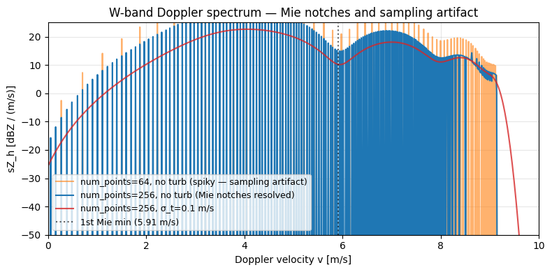
Full Doppler spectrum at 94 GHz (cf. Figure 2)

Running an exponential rain DSD through SpectralIntegrator yields the Mie-modulated Doppler spectrum the paper observes. With enough PSD diameter samples, the Mie minima appear as notches in sZ_h(v) at the velocities we just identified.

Note on diameter sampling

With zero turbulence and too few PSD diameters, the spectrum looks spiky — every tabulated drop lands in a single velocity bin and the bins between stay at zero. This is a sampling artifact, not a physical feature: densify the diameter grid (bump num_points from 64 to 256) or add a hair of turbulence and the spikes collapse into the smooth Mie-modulated spectrum.

def build_rain_W(num_points=256):
    s = Scatterer(wavelength=wl_W, m=m_w_20C[wl_W],
                  Kw_sqr=K_w_sqr[wl_W], ddelt=1e-4, ndgs=2)
    integ = PSDIntegrator()
    integ.D_max = 5.0
    integ.num_points = num_points
    integ.axis_ratio_func = lambda D: 1.0 / dsr_thurai_2007(D)
    integ.geometries = (geom_vert_back,)
    s.psd_integrator = integ
    s.psd_integrator.init_scatter_table(s)
    s.psd = ExponentialPSD(N0=8e3, Lambda=2.2, D_max=5.0)
    return s

rain64  = build_rain_W(num_points=64)
rain256 = build_rain_W(num_points=256)

def run(sc, turb, w=0.0):
    return SpectralIntegrator(
        sc, fall_speed=fall, turbulence=turb, w=w,
        v_min=-1.0, v_max=12.0, n_bins=1024,
        geometry_backscatter=geom_vert_back,
    ).run()

r_sparse = run(rain64,  spectra.NoTurbulence())
r_dense  = run(rain256, spectra.NoTurbulence())
r_turb   = run(rain256, spectra.GaussianTurbulence(0.1))

def dBZ(x):
    return 10 * np.log10(np.maximum(x, 1e-10))

fig, ax = plt.subplots(figsize=(8, 4))
ax.plot(r_sparse.v, dBZ(r_sparse.sZ_h), 'C1-', alpha=0.6,
        label='num_points=64, no turb (spiky — sampling artifact)')
ax.plot(r_dense.v,  dBZ(r_dense.sZ_h),  'C0-',
        label='num_points=256, no turb (Mie notches resolved)')
ax.plot(r_turb.v,   dBZ(r_turb.sZ_h),   'C3-', alpha=0.8,
        label='num_points=256, σ_t=0.1 m/s')
ax.axvline(v_min_obl, color='k', ls=':', alpha=0.6,
           label=f'1st Mie min ({v_min_obl:.2f} m/s)')
ax.set_xlim(0, 10); ax.set_ylim(-50, 25)
ax.set_xlabel('Doppler velocity v [m/s]')
ax.set_ylabel('sZ_h [dBZ / (m/s)]')
ax.set_title('W-band Doppler spectrum — Mie notches and sampling artifact')
ax.legend(fontsize=9); ax.grid(True, alpha=0.3)
fig.tight_layout();

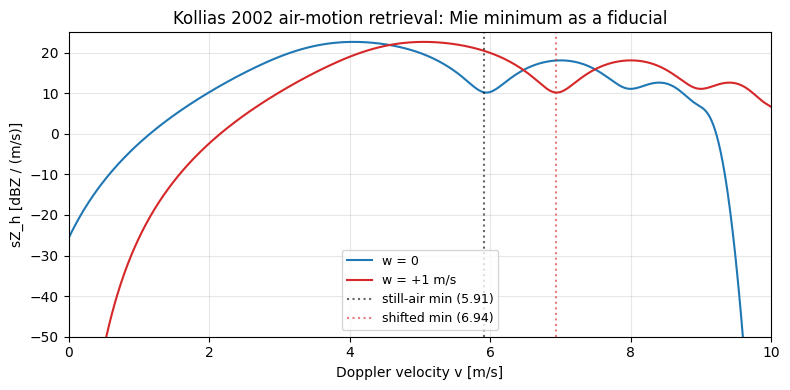
Air-motion retrieval

Simulate a 1 m/s downward air motion (positive w under our convention): the whole spectrum shifts by w, so the first Mie minimum moves from 5.95 m/s to ~6.95 m/s. Subtracting the theoretical still-air Mie-minimum location from the observed one recovers the air motion — this is the Kollias 2002 technique in a nutshell, and it doesn’t depend on knowing the DSD.

r_w = run(rain256, spectra.GaussianTurbulence(0.1), w=1.0)

band = (r_w.v > v_min_obl) & (r_w.v < v_min_obl + 2.5)
v_obs = r_w.v[band][int(np.argmin(r_w.sZ_h[band]))]
w_retrieved = v_obs - v_min_obl
print(f'Prescribed air motion  w = +1.00 m/s (downward)')
print(f'Observed 1st Mie min   v = {v_obs:.2f} m/s')
print(f'Still-air 1st Mie min  v = {v_min_obl:.2f} m/s')
print(f'Retrieved w            = {w_retrieved:+.2f} m/s')

fig, ax = plt.subplots(figsize=(8, 4))
ax.plot(r_turb.v, dBZ(r_turb.sZ_h), 'C0-', label='w = 0')
ax.plot(r_w.v,    dBZ(r_w.sZ_h),    'C3-', label='w = +1 m/s')
ax.axvline(v_min_obl, color='k',  ls=':', alpha=0.6,
           label=f'still-air min ({v_min_obl:.2f})')
ax.axvline(v_obs,     color='C3', ls=':', alpha=0.6,
           label=f'shifted min ({v_obs:.2f})')
ax.set_xlim(0, 10); ax.set_ylim(-50, 25)
ax.set_xlabel('Doppler velocity v [m/s]')
ax.set_ylabel('sZ_h [dBZ / (m/s)]')
ax.set_title('Kollias 2002 air-motion retrieval: Mie minimum as a fiducial')
ax.legend(fontsize=9); ax.grid(True, alpha=0.3)
fig.tight_layout();

Prescribed air motion  w = +1.00 m/s (downward)
Observed 1st Mie min   v = 6.94 m/s
Still-air 1st Mie min  v = 5.91 m/s
Retrieved w            = +1.03 m/s