Tutorial 04 — Oriented ice crystals at W-band

Ice crystals fall with a preferred orientation and a spread of canting angles around it. The orientation PDF captures the spread and feeds directly into the dual-pol observables. This notebook compares the three orientation-averaging strategies rustmatrix ships with: none, fixed-quadrature, and adaptive.

import time
import numpy as np
import matplotlib.pyplot as plt

from rustmatrix import Scatterer, orientation as rs_orient, radar
from rustmatrix.tmatrix_aux import geom_horiz_back, wl_W
from rustmatrix.refractive import mi

One crystal, three averaging schemes

D_eq_mm = 0.5
ice_m = mi(wl_W, 0.9)
pdf = rs_orient.gaussian_pdf(std=20.0, mean=90.0)
base = dict(radius=D_eq_mm/2, wavelength=wl_W, m=ice_m,
            axis_ratio=0.5, ddelt=1e-4, ndgs=2)

schemes = [
    ('single', rs_orient.orient_single, {'or_pdf': pdf}),
    ('fixed 6×12', rs_orient.orient_averaged_fixed,
     {'or_pdf': pdf, 'n_alpha': 6, 'n_beta': 12}),
    ('adaptive', rs_orient.orient_averaged_adaptive, {'or_pdf': pdf}),
]
rows = []
for name, orient, extra in schemes:
    s = Scatterer(**base, **extra)
    s.orient = orient
    s.set_geometry(geom_horiz_back)
    t0 = time.perf_counter()
    zdr = radar.Zdr(s)
    elapsed = time.perf_counter() - t0
    rows.append((name, 10*np.log10(zdr), elapsed))
    print(f'{name:<12} Z_dr = {10*np.log10(zdr):+.4f} dB   ({elapsed*1000:.1f} ms)')

single       Z_dr = -3.1415 dB   (0.3 ms)
fixed 6×12   Z_dr = +1.4293 dB   (3.1 ms)
adaptive     Z_dr = +1.3758 dB   (837.8 ms)

/home/docs/checkouts/readthedocs.org/user_builds/rustmatrix/envs/latest/lib/python3.12/site-packages/scipy/integrate/_quadpack_py.py:1286: IntegrationWarning: The occurrence of roundoff error is detected, which prevents 
  the requested tolerance from being achieved.  The error may be 
  underestimated.
  quad_r = quad(f, low, high, args=args, full_output=self.full_output,
/home/docs/checkouts/readthedocs.org/user_builds/rustmatrix/envs/latest/lib/python3.12/site-packages/scipy/integrate/_quadpack_py.py:1286: IntegrationWarning: The maximum number of subdivisions (50) has been achieved.
  If increasing the limit yields no improvement it is advised to analyze 
  the integrand in order to determine the difficulties.  If the position of a 
  local difficulty can be determined (singularity, discontinuity) one will 
  probably gain from splitting up the interval and calling the integrator 
  on the subranges.  Perhaps a special-purpose integrator should be used.
  quad_r = quad(f, low, high, args=args, full_output=self.full_output,

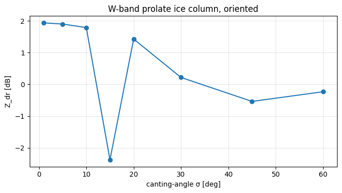
Canting-angle spread sensitivity

Sweep the Gaussian PDF’s std parameter to see how rapidly Z_dr collapses as the orientation spread widens.

stds = np.array([1, 5, 10, 15, 20, 30, 45, 60])
zdrs = np.empty_like(stds, dtype=float)
for i, sd in enumerate(stds):
    s = Scatterer(**base)
    s.orient = rs_orient.orient_averaged_fixed
    s.or_pdf = rs_orient.gaussian_pdf(std=float(sd), mean=90.0)
    s.n_alpha, s.n_beta = 6, 12
    s.set_geometry(geom_horiz_back)
    zdrs[i] = 10 * np.log10(radar.Zdr(s))

fig, ax = plt.subplots(figsize=(7, 4))
ax.plot(stds, zdrs, 'C0-o')
ax.set_xlabel('canting-angle σ [deg]')
ax.set_ylabel('Z_dr [dB]')
ax.set_title('W-band prolate ice column, oriented')
ax.grid(True, alpha=0.3)
fig.tight_layout();