Tutorial 11 — Dual-frequency radar signatures across hydrometeor classes

Reference: Honeyager, R., 2013. Investigating the use of the T-matrix method as a proxy for the discrete dipole approximation, M.S. thesis, Florida State University.

Honeyager’s thesis argues that the T-matrix applied to a size-matched spheroid, with a dielectric built from an ice / air mixing formula at the right volume fraction, reproduces the single-scattering properties of a geometrically-complex hydrometeor (bullet rosettes, plates, dendrites, aggregates) computed with DDA — provided the size parameter χ = 2π r / λ and the effective density are right.

That framing is directly useful for dual-frequency radar work: the whole zoo of ice habits collapses, to first order, onto a two-parameter family (effective density ρ_eff, axis ratio) that rustmatrix already supports via refractive.mi(wl, rho) and the axis_ratio keyword. This notebook walks through four representative hydrometeor classes:

class	ρ_eff [g/cm³]	axis ratio
rain	1.00 (water)	Thurai 2007
low-density aggregate	0.10	0.70
graupel	0.50	0.90
high-density ice	0.90	1.00

and shows how each class signs itself into single-particle σ_b(D), bulk DWR vs. D₀, and the spectral DWR profile sDWR(v).

import numpy as np
import matplotlib.pyplot as plt

from rustmatrix import Scatterer, SpectralIntegrator, radar, spectra
from rustmatrix.psd import ExponentialPSD, PSDIntegrator
from rustmatrix.refractive import m_w_10C, mi
from rustmatrix.tmatrix_aux import (K_w_sqr, dsr_thurai_2007,
                                      geom_vert_back, wl_X, wl_W)

CLASSES = {
    'rain':     dict(rho=1.00, axis_ratio=None),   # Thurai below
    'low-ρ agg':dict(rho=0.10, axis_ratio=0.70),
    'graupel':  dict(rho=0.50, axis_ratio=0.90),
    'high-ρ ice':dict(rho=0.90, axis_ratio=1.00),
}

def refractive_index(wl, cls):
    return m_w_10C[wl] if cls == 'rain' else mi(wl, CLASSES[cls]['rho'])

def class_axis_ratio(cls, D_mm):
    ar = CLASSES[cls]['axis_ratio']
    return (1.0 / dsr_thurai_2007(D_mm)) if ar is None else ar

COLORS = {'rain': 'C0', 'low-ρ agg': 'C2',
          'graupel': 'C1', 'high-ρ ice': 'C3'}

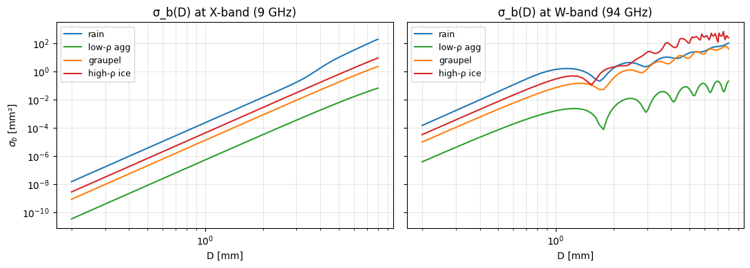
Single-particle σ_b(D) at X and W

For each class, tabulate the single-particle backscatter cross-section at vertical incidence across 0.2–8 mm equivalent diameter. The key effects to watch:

• Rayleigh regime — all classes follow σ_b ∝ D⁶ at small D, but offset vertically by |K(ρ)|² differences. Low-ρ ice sits ~30 dB below water at equal D.

• Non-Rayleigh onset at W-band — the first Mie minimum appears once χ = πD/λ ≈ 1, i.e. D ≈ 1 mm at W-band. That happens for all four classes because χ is set by size, not ρ.

• Mie oscillation amplitude — this is where ρ matters. Denser classes (rain, high-ρ ice) show sharp Mie minima/maxima; low-density aggregates barely oscillate because their refractive index contrast with air is small.

def sigma_b(wl, cls, D_mm):
    s = Scatterer(radius=D_mm/2, wavelength=wl,
                  m=refractive_index(wl, cls),
                  Kw_sqr=K_w_sqr[wl],
                  axis_ratio=class_axis_ratio(cls, D_mm),
                  ddelt=1e-4, ndgs=2)
    s.set_geometry(geom_vert_back)
    return radar.radar_xsect(s)

D_grid = np.linspace(0.2, 8.0, 100)
sigma = {cls: {b: np.array([sigma_b(wl, cls, D) for D in D_grid])
               for b, wl in [('X', wl_X), ('W', wl_W)]}
         for cls in CLASSES}

fig, (axX, axW) = plt.subplots(1, 2, figsize=(11, 4), sharey=True)
for cls in CLASSES:
    axX.loglog(D_grid, sigma[cls]['X'], color=COLORS[cls], label=cls)
    axW.loglog(D_grid, sigma[cls]['W'], color=COLORS[cls], label=cls)
axX.set_title('σ_b(D) at X-band (9 GHz)')
axW.set_title('σ_b(D) at W-band (94 GHz)')
for ax in (axX, axW):
    ax.set_xlabel('D [mm]')
    ax.grid(True, which='both', alpha=0.3)
    ax.legend(fontsize=9)
axX.set_ylabel(r'$\sigma_b$ [mm²]')
fig.tight_layout();

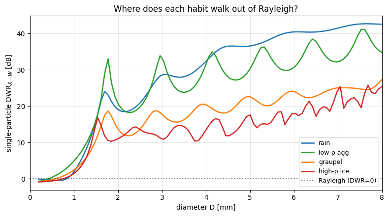
DWR(D) — single-particle dual-wavelength ratio

Re-plotting as DWR(D) = 10·log₁₀(σ_b^X / σ_b^W) collapses the key information: the size where each class first walks out of Rayleigh. This is Honeyager’s thesis Table 2.2 idea generalised to arbitrary habit — the χ parameter that sets Rayleigh validity is hidden inside ρ_eff via the refractive index contrast.

# Equivalent reflectivity normalisation: Ze = λ⁴ / (π⁵ |K_w|²) · σ_b.
# In the Rayleigh regime Ze_X = Ze_W, so DWR_{X-W} = 0 dB; any positive
# excursion is a direct signature of non-Rayleigh scattering at W-band.
def single_Ze(sig, wl, Kw2):
    return wl**4 / (np.pi**5 * Kw2) * sig

fig, ax = plt.subplots(figsize=(8, 4.5))
dwr_curves_1p = {}
for cls in CLASSES:
    zeX = single_Ze(sigma[cls]['X'], wl_X, K_w_sqr[wl_X])
    zeW = single_Ze(sigma[cls]['W'], wl_W, K_w_sqr[wl_W])
    dwr = 10 * np.log10(zeX / zeW)
    dwr_curves_1p[cls] = dwr
    ax.plot(D_grid, dwr, color=COLORS[cls], lw=1.8, label=cls)
ax.axhline(0.0, color='k', ls=':', alpha=0.5, label='Rayleigh (DWR=0)')
ax.set_xlabel('diameter D [mm]')
ax.set_ylabel('single-particle DWR$_{X-W}$ [dB]')
ax.set_title('Where does each habit walk out of Rayleigh?')
ax.set_xlim(0, 8); ax.grid(True, alpha=0.3); ax.legend(fontsize=9)
fig.tight_layout();

print('Approximate D at which single-particle DWR crosses +3 dB:')
for cls, dwr in dwr_curves_1p.items():
    above = np.where(dwr > 3.0)[0]
    label = f'{D_grid[above[0]]:.2f} mm' if len(above) else '> 8 mm (stays Rayleigh)'
    print(f'  {cls:<12}  {label}')

Approximate D at which single-particle DWR crosses +3 dB:
  rain          1.07 mm
  low-ρ agg     0.91 mm
  graupel       1.07 mm
  high-ρ ice    1.15 mm

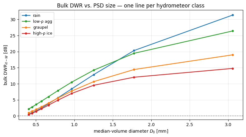
Bulk DWR vs. median-volume diameter D₀

The single-particle curves fold through a PSD in the bulk radar measurement. Hold the habit fixed, sweep the exponential PSD slope Λ (so D₀ = 3.67/Λ varies), and plot the resulting bulk DWR. The curve tells you how sensitive each habit’s dual-frequency signature is to the population-average particle size.

def bulk_Zh(wl, cls, N0, lam, Dmax):
    s = Scatterer(wavelength=wl, m=refractive_index(wl, cls),
                  Kw_sqr=K_w_sqr[wl], ddelt=1e-4, ndgs=2)
    integ = PSDIntegrator()
    integ.D_max = Dmax; integ.num_points = 128
    integ.geometries = (geom_vert_back,)
    if CLASSES[cls]['axis_ratio'] is None:
        integ.axis_ratio_func = lambda D: 1.0 / dsr_thurai_2007(D)
    else:
        s.axis_ratio = CLASSES[cls]['axis_ratio']
    s.psd_integrator = integ
    s.psd_integrator.init_scatter_table(s)
    s.psd = ExponentialPSD(N0=N0, Lambda=lam, D_max=Dmax)
    s.set_geometry(geom_vert_back)
    return radar.refl(s)

# Hold N0 fixed, sweep Λ so D0 = 3.67/Λ spans 0.4–3 mm
Lambdas = np.linspace(1.2, 9.0, 10)   # mm⁻¹
D0s = 3.67 / Lambdas
DMAX = 8.0; N0 = 8e3

dwr_curves = {}
for cls in CLASSES:
    dwr = []
    for lam in Lambdas:
        zX = bulk_Zh(wl_X, cls, N0, lam, DMAX)
        zW = bulk_Zh(wl_W, cls, N0, lam, DMAX)
        dwr.append(10 * np.log10(zX / zW))
    dwr_curves[cls] = np.asarray(dwr)

fig, ax = plt.subplots(figsize=(8, 4.5))
for cls, d in dwr_curves.items():
    ax.plot(D0s, d, color=COLORS[cls], lw=1.8, marker='o',
            markersize=4, label=cls)
ax.axhline(0.0, color='k', ls=':', alpha=0.5)
ax.set_xlabel('median-volume diameter $D_0$ [mm]')
ax.set_ylabel('bulk DWR$_{X-W}$ [dB]')
ax.set_title('Bulk DWR vs. PSD size — one line per hydrometeor class')
ax.grid(True, alpha=0.3); ax.legend(fontsize=9)
fig.tight_layout();

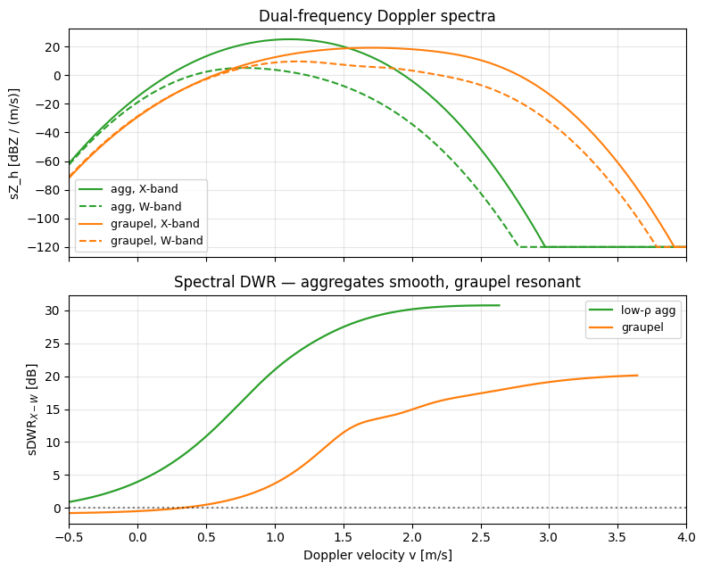
Dual-frequency Doppler spectra — aggregate vs. graupel

Now pull the spectral version together. Two bulk populations that can’t be told apart by reflectivity alone — a low-density aggregate PSD and a graupel PSD tuned to give the same X-band Z_h — show very different sDWR(v) profiles. Aggregates have a mostly-monotonic rise because their σ_b(D) curve stays smooth; graupel’s spectrum carries the Mie-resonance structure of its single-particle σ_b(D) through into velocity space, since every drop size maps deterministically to its own fall speed.

def build(cls, N0, lam, Dmax, wl):
    s = Scatterer(wavelength=wl, m=refractive_index(wl, cls),
                  Kw_sqr=K_w_sqr[wl], ddelt=1e-4, ndgs=2)
    integ = PSDIntegrator()
    integ.D_max = Dmax; integ.num_points = 256
    integ.geometries = (geom_vert_back,)
    if CLASSES[cls]['axis_ratio'] is None:
        integ.axis_ratio_func = lambda D: 1.0 / dsr_thurai_2007(D)
    else:
        s.axis_ratio = CLASSES[cls]['axis_ratio']
    s.psd_integrator = integ
    s.psd_integrator.init_scatter_table(s)
    s.psd = ExponentialPSD(N0=N0, Lambda=lam, D_max=Dmax)
    return s

# PSDs chosen so both give ~moderate snowfall X-band reflectivity.
# Aggregate: low density, broader PSD to Dmax=6 mm.
# Graupel:   medium density, narrower PSD (smaller max D).
agg_X = build('low-ρ agg', N0=2e4, lam=2.0, Dmax=6.0, wl=wl_X)
agg_W = build('low-ρ agg', N0=2e4, lam=2.0, Dmax=6.0, wl=wl_W)
gra_X = build('graupel',   N0=5e3, lam=3.0, Dmax=4.0, wl=wl_X)
gra_W = build('graupel',   N0=5e3, lam=3.0, Dmax=4.0, wl=wl_W)

fall_agg = spectra.fall_speed.locatelli_hobbs_1974_aggregates
fall_gra = spectra.fall_speed.locatelli_hobbs_1974_graupel_hex
turb = spectra.GaussianTurbulence(0.2)
V_MIN, V_MAX = -0.5, 4.0

def run(sc, fall):
    return SpectralIntegrator(
        sc, fall_speed=fall, turbulence=turb,
        v_min=V_MIN, v_max=V_MAX, n_bins=1024,
        geometry_backscatter=geom_vert_back,
    ).run()

r_agg_X = run(agg_X, fall_agg); r_agg_W = run(agg_W, fall_agg)
r_gra_X = run(gra_X, fall_gra); r_gra_W = run(gra_W, fall_gra)

def dBZ(x):
    return 10 * np.log10(np.maximum(x, 1e-12))

print(f'{"population":<15} {"Z_h X [dBZ]":>12} {"Z_h W [dBZ]":>12} '
      f'{"DWR [dB]":>10}')
for name, rX, rW in [('low-ρ agg', r_agg_X, r_agg_W),
                      ('graupel',   r_gra_X, r_gra_W)]:
    zX = 10 * np.log10(np.trapezoid(rX.sZ_h, rX.v))
    zW = 10 * np.log10(np.trapezoid(rW.sZ_h, rW.v))
    print(f'{name:<15} {zX:>12.2f} {zW:>12.2f} {zX - zW:>10.2f}')

fig, (ax1, ax2) = plt.subplots(2, 1, figsize=(8, 6.5), sharex=True)
ax1.plot(r_agg_X.v, dBZ(r_agg_X.sZ_h), 'C2-', label='agg, X-band')
ax1.plot(r_agg_W.v, dBZ(r_agg_W.sZ_h), 'C2--', label='agg, W-band')
ax1.plot(r_gra_X.v, dBZ(r_gra_X.sZ_h), 'C1-', label='graupel, X-band')
ax1.plot(r_gra_W.v, dBZ(r_gra_W.sZ_h), 'C1--', label='graupel, W-band')
ax1.set_ylabel('sZ_h [dBZ / (m/s)]')
ax1.set_title('Dual-frequency Doppler spectra')
ax1.legend(fontsize=9); ax1.grid(True, alpha=0.3)

sdwr_agg = dBZ(r_agg_X.sZ_h) - dBZ(r_agg_W.sZ_h)
sdwr_gra = dBZ(r_gra_X.sZ_h) - dBZ(r_gra_W.sZ_h)
mask_agg = (r_agg_X.sZ_h > 1e-8) & (r_agg_W.sZ_h > 1e-10)
mask_gra = (r_gra_X.sZ_h > 1e-8) & (r_gra_W.sZ_h > 1e-10)
ax2.plot(r_agg_X.v[mask_agg], sdwr_agg[mask_agg], 'C2-',
         lw=1.6, label='low-ρ agg')
ax2.plot(r_gra_X.v[mask_gra], sdwr_gra[mask_gra], 'C1-',
         lw=1.6, label='graupel')
ax2.axhline(0.0, color='k', ls=':', alpha=0.5)
ax2.set_xlabel('Doppler velocity v [m/s]')
ax2.set_ylabel('sDWR$_{X-W}$ [dB]')
ax2.set_title('Spectral DWR — aggregates smooth, graupel resonant')
ax2.set_xlim(V_MIN, V_MAX)
ax2.legend(fontsize=9); ax2.grid(True, alpha=0.3)
fig.tight_layout();

population       Z_h X [dBZ]  Z_h W [dBZ]   DWR [dB]
low-ρ agg              23.25         3.42      19.83
graupel                19.30         9.06      10.25

Takeaway

Following Honeyager 2013’s framing, we’ve used a single T-matrix spheroid code path with four choices of (ρ_eff, axis ratio) to span four physically distinct hydrometeor classes. Two observations pop out that matter for interpreting dual-frequency radar data:

• The size at which DWR departs from zero is set by χ = πD/λ (≈ 1 mm at W-band), not by ρ_eff. But the amplitude and shape of the DWR(D) curve beyond that threshold is a direct fingerprint of ρ_eff: dense classes oscillate strongly, low-ρ aggregates rise smoothly and slowly.

• Bulk DWR sweeps out very different trajectories with D₀, so a single (Z_h, DWR) measurement can be mapped to a habit-dependent D₀ estimate provided you commit to a class — this is exactly the lookup-table strategy that papers like Mason et al. 2019 and Tridon et al. 2019 build their retrievals on.

• Spectral DWR resolves habit ambiguity that bulk DWR can’t: graupel’s Mie resonances appear as wiggles in sDWR(v), while low-ρ aggregates produce a smooth monotonic rise.

Swapping (ρ_eff, axis_ratio) for any other habit class (dendrites, rimed aggregates, hail) is one CLASSES dict entry away.