Tutorial 09 — Reproducing Zhu, Kollias, Yang (2023): particle-inertia spectra#
Reference: Zhu, Z., Kollias, P., and Yang, F., 2023. Particle Inertia Effects on Radar Doppler Spectra Simulation, Atmos. Meas. Tech. Discuss. MATLAB simulator source: https://zenodo.org/records/7897981
The conventional way to get a turbulent radar Doppler spectrum from a drop-size distribution is to convolve the drop reflectivity spectrum with a single Gaussian of width σ_air. Zhu 2023 argues — and shows with a per-drop drag-ODE simulator — that this is wrong: small drops are passive tracers, but large drops are ballistic and under-respond to the small-scale eddies of the wind field. The broadening kernel is diameter-dependent, σ_t(D), and narrows toward the large-drop end.
rustmatrix ships an analytical Stokes-number low-pass response,
InertialZeng2023, implementing this physics family (the Zeng et al.
2023 companion paper):
This notebook reproduces Zhu 2023’s configuration — W-band, ±12 m/s Nyquist, 1024 bins, SNR = 40 dB, exponential warm-rain PSD — and compares conventional Gaussian broadening to the inertia-aware kernel.
import numpy as np
import matplotlib.pyplot as plt

from rustmatrix import Scatterer, SpectralIntegrator, spectra
from rustmatrix.psd import ExponentialPSD, PSDIntegrator
from rustmatrix.refractive import m_w_10C
from rustmatrix.tmatrix_aux import K_w_sqr, geom_vert_back, wl_W

# --- Zhu 2023 configuration ---
V_MIN, V_MAX = -12.0, 12.0
NFFT = 1024
SNR_DB = 40.0
Z_DBZ = 20.0
SIGMA_AIR = 0.289        # std of uniform [-0.5, 0.5] wind field
EPSILON = 1e-2           # dissipation rate (m²/s³)
L_O = 0.1                # integral length scale (m)
Build the W-band rain scatterer and PSD#
Zhu 2023’s MATLAB code uses N(D) = N₀·exp(shape·D_cm)·1e4 m⁻³ µm⁻¹ with N₀ = 0.08 and shape = -20. In rustmatrix’s mm-based units this is N(D_mm) = 8×10⁵ · exp(-2·D_mm) m⁻³ mm⁻¹, truncated at D_max=4 mm.
s = Scatterer(wavelength=wl_W, m=m_w_10C[wl_W],
              Kw_sqr=K_w_sqr[wl_W], ddelt=1e-4, ndgs=2)
integ = PSDIntegrator()
integ.D_max = 4.0; integ.num_points = 128
integ.geometries = (geom_vert_back,)
s.psd_integrator = integ
s.psd_integrator.init_scatter_table(s)
s.psd = ExponentialPSD(N0=8e5, Lambda=2.0, D_max=4.0)
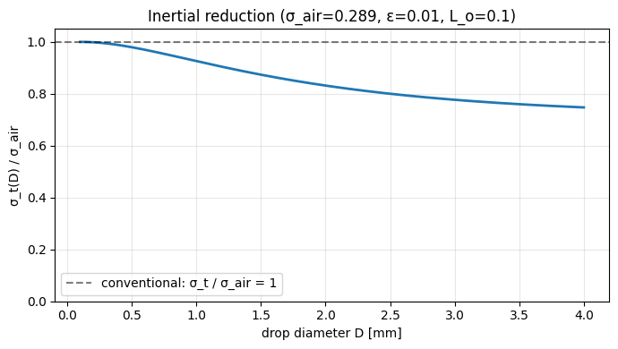
The inertial reduction factor σ_t(D) / σ_air#
At fixed σ_air and ε, the reduction factor depends only on D through the particle relaxation time τ_p(D) = v_t(D)/g. This plot is the physical crux of Zhu 2023 — large drops experience less-effective turbulence broadening than small drops.
zeng = spectra.InertialZeng2023(sigma_air=SIGMA_AIR,
                                 epsilon=EPSILON, L_o=L_O)
D_plot = np.linspace(0.1, 4.0, 200)
fig, ax = plt.subplots(figsize=(7, 4))
ax.plot(D_plot, zeng(D_plot) / SIGMA_AIR, 'C0-', lw=2)
ax.axhline(1.0, color='k', ls='--', alpha=0.5,
           label='conventional: σ_t / σ_air = 1')
ax.set_xlabel('drop diameter D [mm]')
ax.set_ylabel('σ_t(D) / σ_air')
ax.set_title(f'Inertial reduction (σ_air={SIGMA_AIR}, '
             f'ε={EPSILON}, L_o={L_O})')
ax.legend(); ax.grid(True, alpha=0.3)
ax.set_ylim(0.0, 1.05)
fig.tight_layout();
Run two spectra: conventional vs. inertia-aware#
Both use the same fall-speed model, velocity grid, and noise floor. The only difference is the turbulence kernel — constant σ_air vs. σ_t(D) from Zeng 2023.
# Receiver noise: SNR = 40 dB over 20 dBZ reference.
noise = 10 ** (Z_DBZ / 10.0) / 10 ** (SNR_DB / 10.0)

common = dict(
    fall_speed=spectra.fall_speed.atlas_srivastava_sekhon_1973,
    v_min=V_MIN, v_max=V_MAX, n_bins=NFFT,
    geometry_backscatter=geom_vert_back,
    noise=noise,
)

conv = SpectralIntegrator(s,
    turbulence=spectra.GaussianTurbulence(SIGMA_AIR),
    **common,
).run()

iner = SpectralIntegrator(s,
    turbulence=spectra.InertialZeng2023(
        sigma_air=SIGMA_AIR, epsilon=EPSILON, L_o=L_O),
    **common,
).run()

print(f'Conventional integrated Z_h = '
      f'{10*np.log10(np.trapezoid(conv.sZ_h, conv.v)):.2f} dBZ')
print(f'Inertia-aware integrated Z_h = '
      f'{10*np.log10(np.trapezoid(iner.sZ_h, iner.v)):.2f} dBZ')
print(f'Noise floor              = '
      f'{noise:.4f} mm⁶/m³ ('
      f'{10*np.log10(noise / (V_MAX - V_MIN)):.2f} '
      f'dBZ / (m/s))')
Conventional integrated Z_h = 47.00 dBZ
Inertia-aware integrated Z_h = 47.00 dBZ
Noise floor              = 0.0100 mm⁶/m³ (-33.80 dBZ / (m/s))
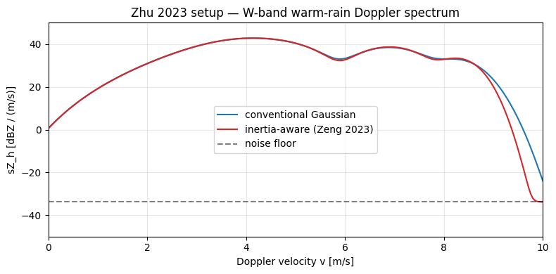
Spectrum comparison in dBZ#
On a log scale the inertia correction visibly narrows the spectrum near the fall-speed of the largest drops (the right-hand tail). The total power integrates to the same reflectivity — this is a redistribution of spectral shape, not a gain change.
def dBZ(x):
    return 10 * np.log10(np.maximum(x, 1e-12))

fig, ax = plt.subplots(figsize=(8, 4))
ax.plot(conv.v, dBZ(conv.sZ_h), 'C0-',
        label='conventional Gaussian')
ax.plot(iner.v, dBZ(iner.sZ_h), 'C3-',
        label='inertia-aware (Zeng 2023)')
ax.axhline(dBZ(noise / (V_MAX - V_MIN)), color='k',
           ls='--', alpha=0.5, label='noise floor')
peak = max(dBZ(conv.sZ_h).max(), dBZ(iner.sZ_h).max())
ax.set_xlim(0, 10)
ax.set_ylim(-50, np.ceil(peak / 5.0) * 5.0 + 5)
ax.set_xlabel('Doppler velocity v [m/s]')
ax.set_ylabel('sZ_h [dBZ / (m/s)]')
ax.set_title('Zhu 2023 setup — W-band warm-rain Doppler spectrum')
ax.legend(); ax.grid(True, alpha=0.3)
fig.tight_layout();
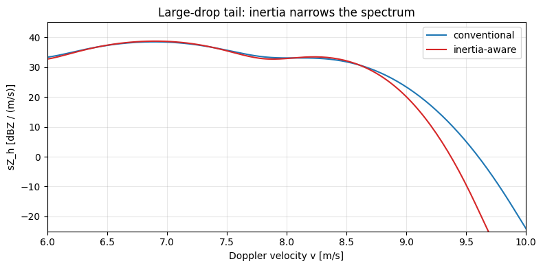
Zoom on the large-drop tail#
Narrowing is most visible between v ≈ 7–9 m/s, where the fastest drops land. Zhu 2023’s Lagrangian drop-tracking simulator produces the same qualitative signature (their Fig. 3–5).
fig, ax = plt.subplots(figsize=(8, 4))
ax.plot(conv.v, dBZ(conv.sZ_h), 'C0-', label='conventional')
ax.plot(iner.v, dBZ(iner.sZ_h), 'C3-', label='inertia-aware')
ax.set_xlim(6, 10)
tail_peak = max(dBZ(conv.sZ_h[(conv.v > 6) & (conv.v < 10)]).max(),
                dBZ(iner.sZ_h[(iner.v > 6) & (iner.v < 10)]).max())
ax.set_ylim(-25, np.ceil(tail_peak / 5.0) * 5.0 + 5)
ax.set_xlabel('Doppler velocity v [m/s]')
ax.set_ylabel('sZ_h [dBZ / (m/s)]')
ax.set_title('Large-drop tail: inertia narrows the spectrum')
ax.legend(); ax.grid(True, alpha=0.3)
fig.tight_layout();