Tutorial 10 — Supercooled liquid water vs. snow at cloud-radar frequencies#
Reference: Billault-Roux, A.-C., Georgakaki, P., Grazioli, J., Romanens, G., Sotiropoulou, G., Phillips, V., Nenes, A., and Berne, A., 2023. Distinct secondary ice production processes observed in radar Doppler spectra: insights from a case study, Atmos. Chem. Phys., 23, 10207–10234 (doi:10.5194/acp-23-10207-2023).
Mixed-phase cloud volumes contain supercooled liquid droplets (SLW) and ice particles side by side. The two populations have completely different scattering and fall-speed signatures:
SLW: small (≲200 µm), spherical, cold refractive index of water, falls at a few cm/s. Rayleigh at both X- and W-band ⇒ very low Z_h, Z_dr ≈ 0 dB, no polarimetric signature.
Snow: millimetre-scale oblate low-density aggregates, falls at ~0.5–1 m/s. Moderately non-Rayleigh at W-band ⇒ higher Z_h, small positive Z_dr from the habit anisotropy.
This notebook builds dedicated scatterers for each population, shows
their σ_b(D) and bulk radar observables at X and W band, and then
combines them in a HydroMix to produce the bimodal Doppler spectrum
that motivates the Billault-Roux et al. case-study analysis.
import numpy as np
import matplotlib.pyplot as plt

from rustmatrix import (HydroMix, MixtureComponent, Scatterer,
                         SpectralIntegrator, radar, spectra)
from rustmatrix.psd import ExponentialPSD, GammaPSD, PSDIntegrator
from rustmatrix.refractive import m_w_0C, mi
from rustmatrix.tmatrix_aux import (K_w_sqr, geom_vert_back,
                                      wl_X, wl_W)
Build a supercooled-liquid-water scatterer#
Small spherical drops (D in 10–200 µm), refractive index at 0°C,
log-normal-ish gamma PSD centred around 30 µm. We use mm units
throughout to match rustmatrix conventions.
SLW_DMAX = 0.2  # mm

def build_slw(wl):
    s = Scatterer(wavelength=wl, m=m_w_0C[wl],
                  Kw_sqr=K_w_sqr[wl], axis_ratio=1.0,
                  ddelt=1e-4, ndgs=2)
    integ = PSDIntegrator()
    integ.D_max = SLW_DMAX
    integ.num_points = 128
    integ.geometries = (geom_vert_back,)
    s.psd_integrator = integ
    s.psd_integrator.init_scatter_table(s)
    # Gamma PSD: D0 = 0.03 mm (30 µm), Nw = 1e11 m⁻³ mm⁻¹, μ = 4
    s.psd = GammaPSD(D0=0.03, Nw=1e11, mu=4, D_max=SLW_DMAX)
    return s

slw_X = build_slw(wl_X)
slw_W = build_slw(wl_W)
Build a snow scatterer (low-density oblate aggregates)#
SNOW_DMAX = 8.0
RHO_SNOW = 0.2
AXIS_SNOW = 0.6

def build_snow(wl):
    s = Scatterer(wavelength=wl, m=mi(wl, RHO_SNOW),
                  Kw_sqr=K_w_sqr[wl], axis_ratio=AXIS_SNOW,
                  ddelt=1e-4, ndgs=2)
    integ = PSDIntegrator()
    integ.D_max = SNOW_DMAX
    integ.num_points = 256
    integ.geometries = (geom_vert_back,)
    s.psd_integrator = integ
    s.psd_integrator.init_scatter_table(s)
    s.psd = ExponentialPSD(N0=5e3, Lambda=1.0, D_max=SNOW_DMAX)
    return s

snow_X = build_snow(wl_X)
snow_W = build_snow(wl_W)
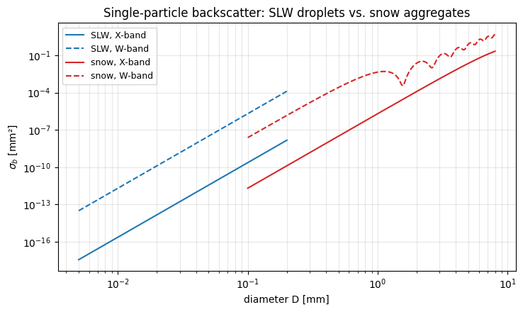
σ_b(D) — Rayleigh vs. Mie across the two populations#
def sigma_b(wl, D_mm, m, axis_ratio):
    s = Scatterer(radius=D_mm/2, wavelength=wl, m=m,
                  Kw_sqr=K_w_sqr[wl], axis_ratio=axis_ratio,
                  ddelt=1e-4, ndgs=2)
    s.set_geometry(geom_vert_back)
    return radar.radar_xsect(s)

D_slw = np.linspace(0.005, SLW_DMAX, 60)
D_snow = np.linspace(0.1, SNOW_DMAX, 200)

sb_slw_X = np.array([sigma_b(wl_X, d, m_w_0C[wl_X], 1.0) for d in D_slw])
sb_slw_W = np.array([sigma_b(wl_W, d, m_w_0C[wl_W], 1.0) for d in D_slw])
sb_snow_X = np.array([sigma_b(wl_X, d, mi(wl_X, RHO_SNOW), AXIS_SNOW)
                       for d in D_snow])
sb_snow_W = np.array([sigma_b(wl_W, d, mi(wl_W, RHO_SNOW), AXIS_SNOW)
                       for d in D_snow])

fig, ax = plt.subplots(figsize=(7.5, 4.5))
ax.loglog(D_slw, sb_slw_X, 'C0-',  label='SLW, X-band')
ax.loglog(D_slw, sb_slw_W, 'C0--', label='SLW, W-band')
ax.loglog(D_snow, sb_snow_X, 'C3-',  label='snow, X-band')
ax.loglog(D_snow, sb_snow_W, 'C3--', label='snow, W-band')
ax.set_xlabel('diameter D [mm]')
ax.set_ylabel(r'$\sigma_b$ [mm²]')
ax.set_title('Single-particle backscatter: SLW droplets vs. snow aggregates')
ax.legend(fontsize=9); ax.grid(True, which='both', alpha=0.3)
fig.tight_layout();
Bulk radar observables at X and W band#
Z_h(SLW) is ~40+ dB below Z_h(snow) even though the droplet concentration is high — the D⁶ Rayleigh penalty at 30-µm scale kills the signal. Z_dr is zero for SLW (spheres) but positive for snow (oblate). Dual-wavelength ratio DWR = Z_X − Z_W is near zero for SLW and positive for snow (non-Rayleigh at W-band).
def bulk(s):
    s.set_geometry(geom_vert_back)
    return 10 * np.log10(radar.refl(s))

print(f'{"":<10} {"Z_h X [dBZ]":>12} {"Z_h W [dBZ]":>12} '
      f'{"DWR [dB]":>10}')
for name, sX, sW in [('SLW',  slw_X,  slw_W),
                      ('snow', snow_X, snow_W)]:
    zX = bulk(sX); zW = bulk(sW)
    print(f'{name:<10} {zX:>12.2f} {zW:>12.2f} {zX - zW:>10.2f}')
            Z_h X [dBZ]  Z_h W [dBZ]   DWR [dB]
SLW               -9.38        -9.80       0.42
snow              41.49        16.85      24.65
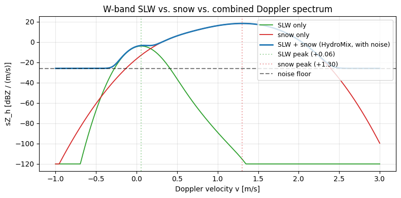
Bimodal Doppler spectrum of the SLW + snow mixture#
A HydroMix with per-component fall-speed and turbulence captures
the two populations cleanly: SLW pins to v ≈ 0 with a narrow spread,
snow sits near 0.5–1.0 m/s with a broader tail. Plotted in dBZ space
the two modes are clearly separable even with realistic noise.
# Use W-band for the spectrum — best velocity-wise resolution of the
# SLW mode, and non-Rayleigh snow signature is most evident here.
mix = HydroMix([
    MixtureComponent(slw_W,  slw_W.psd,  'slw'),
    MixtureComponent(snow_W, snow_W.psd, 'snow'),
])

integ = SpectralIntegrator(
    mix,
    component_kinematics={
        'slw':  (lambda D: 0.003 * (D / 0.01) ** 2,
                 spectra.GaussianTurbulence(0.1)),
        'snow': (spectra.fall_speed.locatelli_hobbs_1974_aggregates,
                 spectra.GaussianTurbulence(0.2)),
    },
    v_min=-1.0, v_max=3.0, n_bins=1024,
    geometry_backscatter=geom_vert_back,
    noise='realistic',
).run()

def dBZ(x):
    return 10 * np.log10(np.maximum(x, 1e-12))

# Run each population on its own (no noise) so each mode's true peak
# is unambiguous. The HydroMix spectrum is dominated by snow (~50 dB
# louder than SLW), so looking for the SLW peak on the combined,
# noise-added spectrum would just pick up the snow tail crossing
# through the near-zero velocity range.
slw_only = SpectralIntegrator(
    slw_W,
    fall_speed=lambda D: 0.003 * (D / 0.01) ** 2,
    turbulence=spectra.GaussianTurbulence(0.1),
    v_min=-1.0, v_max=3.0, n_bins=1024,
    geometry_backscatter=geom_vert_back,
).run()
snow_only = SpectralIntegrator(
    snow_W,
    fall_speed=spectra.fall_speed.locatelli_hobbs_1974_aggregates,
    turbulence=spectra.GaussianTurbulence(0.2),
    v_min=-1.0, v_max=3.0, n_bins=1024,
    geometry_backscatter=geom_vert_back,
).run()

v_slw  = slw_only.v[int(np.argmax(slw_only.sZ_h))]
v_snow = snow_only.v[int(np.argmax(snow_only.sZ_h))]
print(f'SLW mode peak  v = {v_slw:+.3f} m/s')
print(f'snow mode peak v = {v_snow:+.3f} m/s')

fig, ax = plt.subplots(figsize=(8, 4))
ax.plot(slw_only.v, dBZ(slw_only.sZ_h), 'C2-', lw=1.3, label='SLW only')
ax.plot(snow_only.v, dBZ(snow_only.sZ_h), 'C3-', lw=1.3, label='snow only')
ax.plot(integ.v, dBZ(integ.sZ_h), 'C0-', lw=2.0,
        label='SLW + snow (HydroMix, with noise)')
ax.axvline(v_slw,  color='C2', alpha=0.4, ls=':',
           label=f'SLW peak ({v_slw:+.2f})')
ax.axvline(v_snow, color='C3', alpha=0.4, ls=':',
           label=f'snow peak ({v_snow:+.2f})')
ax.axhline(dBZ(integ.noise_h / (integ.v[-1] - integ.v[0])),
           color='k', ls='--', alpha=0.5, label='noise floor')
ax.set_xlabel('Doppler velocity v [m/s]')
ax.set_ylabel('sZ_h [dBZ / (m/s)]')
ax.set_title('W-band SLW vs. snow vs. combined Doppler spectrum')
ax.legend(fontsize=9, loc='upper right'); ax.grid(True, alpha=0.3)
fig.tight_layout();
SLW mode peak  v = +0.056 m/s
snow mode peak v = +1.303 m/s
Takeaway#
The Billault-Roux et al. 2023 case study relies on the spectral
separability demonstrated here: a narrow near-zero Doppler peak is
SLW, a broader fall-velocity peak is ice; the polarimetric spectral
variables further distinguish columnar (high SLDR) from planar and
aggregated ice. With the two populations built as independent
rustmatrix scatterers you can plug them into HydroMix and recover
bulk radar observables that match what a vertically-pointing radar
would measure, or analyse the spectral signatures by looking at the
individual modes.