Tutorial 05 — One PSD, six radar bands

Retrieval algorithms that use more than one frequency need a forward model that works across the whole instrument suite. This notebook runs the same moderate-convective gamma PSD through rustmatrix at S, C, X, Ku, Ka, and W band and plots the frequency response of the dual-pol observables.

import numpy as np
import matplotlib.pyplot as plt

from rustmatrix import Scatterer, radar, psd as rs_psd
from rustmatrix.tmatrix_aux import (dsr_thurai_2007, geom_horiz_back,
                                      geom_horiz_forw, K_w_sqr,
                                      wl_S, wl_C, wl_X, wl_Ku,
                                      wl_Ka, wl_W)
from rustmatrix.refractive import m_w_20C

BANDS = [('S', wl_S), ('C', wl_C), ('X', wl_X),
         ('Ku', wl_Ku), ('Ka', wl_Ka), ('W', wl_W)]

Run the six bands

def run(wl):
    s = Scatterer(wavelength=wl, m=m_w_20C[wl],
                  Kw_sqr=K_w_sqr[wl], ddelt=1e-4, ndgs=2)
    integ = rs_psd.PSDIntegrator()
    integ.D_max = 8.0
    integ.num_points = 64
    integ.axis_ratio_func = lambda D: 1.0 / dsr_thurai_2007(D)
    integ.geometries = (geom_horiz_back, geom_horiz_forw)
    s.psd_integrator = integ
    s.psd_integrator.init_scatter_table(s)
    s.psd = rs_psd.GammaPSD(D0=1.5, Nw=8e3, mu=4)
    s.set_geometry(geom_horiz_back)
    Zh = 10 * np.log10(radar.refl(s))
    Zdr = 10 * np.log10(radar.Zdr(s))
    s.set_geometry(geom_horiz_forw)
    return Zh, Zdr, radar.Kdp(s), radar.Ai(s)

Zh = {}; Zdr = {}; Kdp = {}; Ai = {}
for name, wl in BANDS:
    Zh[name], Zdr[name], Kdp[name], Ai[name] = run(wl)
    print(f'{name:<3} Z_h={Zh[name]:6.2f}  Z_dr={Zdr[name]:+.3f}  '
          f'K_dp={Kdp[name]:+.3f}  A_i={Ai[name]:.4f}')

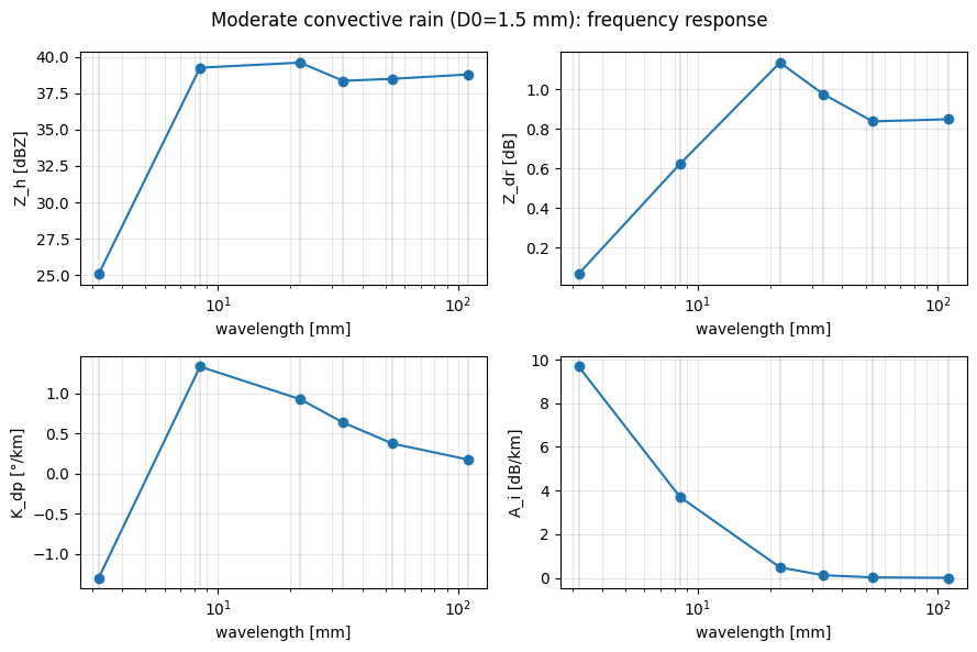
S   Z_h= 38.78  Z_dr=+0.848  K_dp=+0.171  A_i=0.0034
C   Z_h= 38.48  Z_dr=+0.838  K_dp=+0.372  A_i=0.0233
X   Z_h= 38.34  Z_dr=+0.976  K_dp=+0.634  A_i=0.1213
Ku  Z_h= 39.59  Z_dr=+1.135  K_dp=+0.926  A_i=0.4818
Ka  Z_h= 39.24  Z_dr=+0.623  K_dp=+1.332  A_i=3.7075
W   Z_h= 25.10  Z_dr=+0.067  K_dp=-1.301  A_i=9.6771

Plot the frequency response

names = [b[0] for b in BANDS]
wls = np.array([b[1] for b in BANDS])
fig, axes = plt.subplots(2, 2, figsize=(9, 6))
axes[0, 0].semilogx(wls, [Zh[n] for n in names], 'o-'); axes[0, 0].set_ylabel('Z_h [dBZ]')
axes[0, 1].semilogx(wls, [Zdr[n] for n in names], 'o-'); axes[0, 1].set_ylabel('Z_dr [dB]')
axes[1, 0].semilogx(wls, [Kdp[n] for n in names], 'o-'); axes[1, 0].set_ylabel('K_dp [°/km]')
axes[1, 1].semilogx(wls, [Ai[n] for n in names], 'o-'); axes[1, 1].set_ylabel('A_i [dB/km]')
for ax, label in zip(axes.flat, names*4):
    ax.set_xlabel('wavelength [mm]')
    ax.grid(True, alpha=0.3, which='both')
    for name, wl in BANDS:
        ax.axvline(wl, color='k', alpha=0.1)
fig.suptitle('Moderate convective rain (D0=1.5 mm): frequency response')
fig.tight_layout();